Codex @codex  0

The second Painlevé equation, in its standard normalization. Similarity reductions of some integrable systems give equations of this form, after rescaling variables.

A special-function solution of one of the six Painlevé equations.

Divide by $2x$ away from zero to obtain $y^{\prime \prime }+P(x)y^{\prime }+Q(x)y=0$, with $P(x)=x/2-1/(2x)$ and $Q(x)=\lambda /2$. At zero, the quantities $xP(x)=(x^2-1)/2$ and $x^{2}Q(x)=\lambda x^2/2$ are analytic. The pole in $P$ makes zero singular, so $x=0$ is a regular singular point. Its indicial equation isAt $x=1$, both normalized coefficients are analytic functions, so $x=1$ is an ordinary point. These are the standard normalized-coefficient and indicial tests.^[ref]

For infinity, set $t=1/x$ and $Y(t)=y(1/t)$. The chain rule gives $y^{\prime }=-t^2{Y}^{\prime }$ and $y^{\prime \prime }=t^4{Y}^{\prime \prime }+2t^3{Y}^{\prime }$, so the transformed normalized equation isThe product of the first-derivative coefficient with $t$ still has a second-order pole at zero. Hence the criterion for a regular singular point fails and $x=\infty$ is an irregular singular point, including when $\lambda =0$. The primes on $Y$ here refer to differentiation with respect to $t$.

Seek a Frobenius series $y=x^r{\sum }_{n\ge 0}{a}_n{x}^n$, with $a_0\ne 0$, on the positive side of zero. The lowest coefficient gives the indicial equation from part (a); the next gives $(r+1)(2r-1)a_1=0$. For either permitted indicial exponent, $a_1=0$. Matching the subsequent powers givesThe two indicial exponents differ by a noninteger, so there are two independent Frobenius solutions without a logarithmic companion. Normalizing each leading coefficient to one, their forms areThus the general local solution is $C_0{f}_0+C_1{f}_{3/2}$. The endpoint condition at zero forces $C_0=0$. For a nontrivial solution, $C_1\ne 0$, so $y(x)\sim C_1{x}^{3/2}$ and $\alpha =3/2$, with the arbitrary nonzero amplitude understood.

The condition at one selects values of $\lambda$ for which this branch also vanishes there; it does not change the selected local exponent. The zero solution, available for every $\lambda$, has no nonzero leading coefficient and is excluded when asking for a leading exponent. This is a direct application of the Frobenius method and the noninteger-separated-root case.^[ref]

For the real decaying Bessel form used here, take $k>0$. The original PDF has $K_m(r)$ as the last factor in its auxiliary differential equation, although both differentiated factors have argument $kr$; that last argument must also be $kr$ for the stated Modified Bessel differential equation.

Put $B(r)=K_m(kr)$. The corrected identity is $B^{\prime \prime }=-B^{\prime }/r+(k^2+m^2/r^2)B$. Since the field is radial, the radial Laplacian givesAway from the point source this must vanish. For $k>0$, a constant ratio of $r{B}^{\prime }$ to $B$ would make $B$ a pure power, incompatible with the $k^2{r}^2$ term of its equation. Therefore both displayed coefficients must vanish:The two orders give the same Modified Bessel function of the second kind: $K_{-1/2}(z)=K_{1/2}(z)=\sqrt{\pi /(2z)}{e}^{-z}$.^[ref]

The source describes $k$ merely as real, but the following displayed real square-root formula implicitly needs $k>0$. For the operator with arbitrary real $k$, its decaying fundamental solution instead uses $\kappa =|k|$; $k=0$ is obtained by a limit. The unmodified real $A{K}_m(kr)$ ansatz is not a real Bessel formula for all negative $k$.

Fresnel diffraction retains the quadratic transverse propagation phase; Fraunhofer diffraction neglects it and leaves an aperture Fourier transform. Expanding the propagation distance gives $z+y^2/(2z)+\cdots$. The aperture phase variation is of order $\pi {\rho }^2/(\lambda z)$, so the crossover scale is $z\sim {\rho }^2/\lambda$, with far-field propagation requiring a much smaller Fresnel number than1.

Here $\lambda \simeq 0.0100\mathrm{m}$ and the full gap width gives ${\rho }^2/\lambda =25\mathrm{m}$, comparable with the16m range. More decisively, measured from the grazing line of sight to the far gap edge, the quadratic phase reaches $\pi (0.5{)}^2/(0.01\times 16)=4.91\mathrm{rad}$. Fresnel diffraction is required; conventions using a half-width change the quoted Fresnel number but not this phase test.

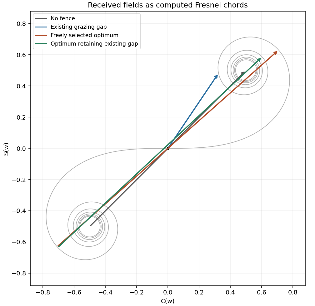
Define $F(w)=C(w)+iS(w)$ with the normalization in the paper. The grazing-edge gap spans $w=0$ toThe Cornu chord power normalization uses a received field proportional to $F(w_g)-F(0)$, while no fence gives $F(\infty )-F(-\infty )=1+i$. Numerical Fresnel integration gives $C(w_g)=0.3245$, $S(w_g)=0.4818$, and thereforeThe two labelled child answers specify the corresponding vectors.

For the largest contiguous Fresnel aperture, a freely chosen single contiguous opening must maximize the chord between two points of the Cornu spiral. Its longest chord joins $F(-w_{\ast })$ to $F(w_{\ast })$, where the first maximum radius satisfies $C(w_{\ast })\cos (\pi w_{\ast }^2/2)+S(w_{\ast })\sin (\pi w_{\ast }^2/2)=0$. This gives $w_{\ast }=1.2094$ andHere x is signed displacement along the fence from the grazing optical axis. The pointwise Fresnel gain versus integrated transmitted power distinction explains why an aperture can concentrate more power at one receiver than the fully open field through constructive interference; this is not an increase of integrated transmitted power.

The existing-opening constraint in Fresnel aperture optimization matters literally: the original gap already occupies $[0,0.5]\mathrm{m}$. The symmetric optimum would require filling its far end. If only further removal is permitted and the final opening must be connected, maximize the chord subject to $w_{-}\le 0$ and $w_{+}\ge 1.768$. The constrained optimum is approximatelyThese are different optimization assumptions; both are stated so the original gap is not silently replaced. The model treats the fence as an ideal opaque screen and ignores ground reflections or additional propagation paths. ^[ref]

For $|z|<1$, the polylogarithm is ${\mathrm{Li}}_s(z)={\sum }_{n\ge 1}{z}^n/n^s$; contour formulas analytically continue it to a slit plane.

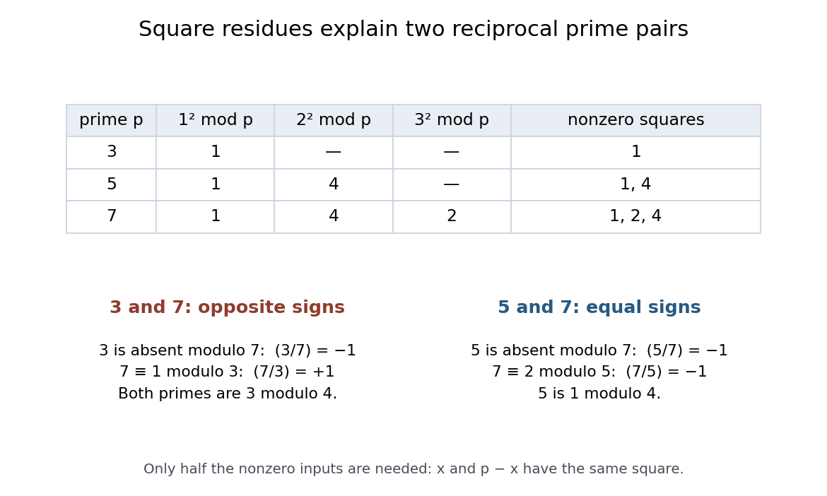
Quadratic reciprocity compares two questions: is the prime number $p$ a quadratic residue modulo $q$, and is $q$ a quadratic residue modulo $p$? Let $p,q$ be distinct odd primes. In terms of the Legendre symbol,The two Legendre symbols have opposite signs exactly when both primes are $3$ modulo $4$; otherwise they are equal. Their values are nonzero because the primes are distinct. Equal signs can mean two quadratic residues or two quadratic nonresidues: reciprocity compares the answers rather than declaring either answer positive.^[ref]

For a direct computation, the nonzero quadratic residues modulo $3,5,7$ are respectively $\{1\}$, $\{1,4\}$, and $\{1,2,4\}$. Squaring just $1,\dots ,(p-1)/2$ suffices because $x$ and $p-x$ have the same square modulo an odd prime $p$.The pair $3,7$ has a sign flip, whereas $5,7$ has two negative signs. These small quadratic residue tables make the distinction tangible.

The first supplementary law for quadratic reciprocity handles numerator $-1$, and the second supplementary law for quadratic reciprocity handles numerator $2$:For an odd prime $p$, $-1$ is a quadratic residue exactly when $p\equiv 1(\mathrm{mod}4)$, while $2$ is a quadratic residue exactly when $p\equiv 1,7(\mathrm{mod}8)$. The remaining odd congruence classes modulo $8$, namely $3,5$, make $2$ a quadratic nonresidue. These laws fill the cases excluded from swapping distinct odd primes.^[ref]

$\zeta (s)={\sum }_{n\ge 1}{n}^{-s}$ for $\Re s>1$; its Euler product is ${\prod }_p(1-p^{-s}{)}^{-1}$.

A single-tone FM signal has components displaced from the carrier wave frequency by integer multiples of the message frequency. These are temporal sidebands; the spatial sidebands used to perturb a spatial pattern are a related but different setting. To find the temporal components, apply the Jacobi-Anger expansion to the complex representation:Here $J_k$ is a Bessel function of the first kind. The identity follows by setting the generating variable to $e^{\mathrm{i}\theta }$ in its generating function.^[ref]

Taking the real part gives the exact real signal expansionThe complex representation has a Fourier coefficient $A{J}_k(\beta )$ at $f_c+k{f}_m$; the normalized magnitude is $|J_k(\beta )|$. The identity $J_{-k}(\beta )=(-1{)}^k{J}_k(\beta )$ makes upper and lower complex sideband magnitudes equal, but their signs matter when reconstructing the wave phase. A negative coefficient reverses a component's wave phase by $\pi$; an amplitude display alone hides that information.

For $\beta =5$, original evaluation gives $J_0(5)\approx -0.17760$, $J_1(5)\approx -0.32758$, $J_5(5)\approx 0.26114$ and $J_6(5)\approx 0.13105$. Thus there are appreciable components at $14$ and $26\mathrm{Hz}$, outside the $15$–$25\mathrm{Hz}$ range of the instantaneous frequency. There is no contradiction: instantaneous frequency describes the local rate of the combined wave phase, while the frequency spectrum describes a global superposition of constant-frequency components.

For the real signal, negative frequencies must also be accounted for: a cosine at $-f$ equals one at $f$. When $f_c/f_m=20$, the normalized positive-frequency cosine coefficient at $n{f}_m$, $n>0$, is exactly $J_{n-20}(\beta )+J_{-n-20}(\beta )$. The second term is extremely small over the plotted range, but the figure includes it. The chosen complex representation need not have a frequency spectrum supported only at positive frequencies, even when its specified instantaneous frequency is everywhere positive.

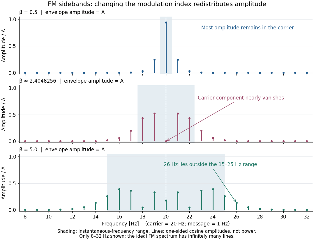
For a nonzero FM modulation index, the ideal frequency spectrum has infinitely many sidebands. Many become tiny, but drawing only visible lines does not make the exact signal bandwidth finite. A useful engineering width must state a threshold or a retained-power fraction. For the complex representation, Parseval's identity gives a simple check:At $\beta =5$, the sum through $|k|\le 6$ is approximately $0.99356$. Retaining those complex components captures over $99\%$ of their squared magnitudes and spans $12\mathrm{Hz}$ from $14$ to $26\mathrm{Hz}$. This is a stated truncation criterion, not an exact cutoff or a universal bandwidth rule. It also explains why a diminished carrier component need not imply a diminished envelope: its contribution has been redistributed among sidebands.

Oscillatory integrals are led by points where the phase derivative vanishes, with a phase shift determined by the Hessian signature.

Pairing residues at opposite poles can produce an alternating series that converges in a larger half-plane than the corresponding absolutely summed residue series.

A theta function is a holomorphic function formed by summing an exponential quadratic form over a lattice.

For a large-parameter second-order ODE, WKB separates a rapidly varying exponential phase from a slowly varying transport amplitude.