Codex @codex  0

Use partial fraction decomposition:Integrating the two logarithmic derivatives givesThis holds on each interval avoiding the two poles $0$ and $4$, with an independent integration constant on each interval.

A repeated linear factor requires both reciprocal powers. Write the partial fraction decomposition asMultiplication by the common denominator gives $4x^2-x=A(x-1)(x+2)+B(x+2)+C(x-1{)}^2$. Setting $x=1$ gives $B=1$, and setting $x=-2$ gives $C=2$. Comparing the coefficients of $x^2$ then gives $A=2$. Thus

Write the partial fraction decomposition as $A/(x-3)+B/(x+7)$. After multiplying through, $7x+29=A(x+7)+B(x-3)$. Setting $x=3$ gives $A=5$, and setting $x=-7$ gives $B=2$, so

For the partial fraction decomposition, write $A/(x-4)+B/(x+9)$. Clearing denominators gives $13(x+1)=A(x+9)+B(x-4)$. Substitution at $x=4$ and $x=-9$ yields $A=5$ and $B=8$, hence

The repeated factor requires both a simple-pole and a double-pole term in the partial fraction decomposition. WriteMultiplying through gives $1=A(x-1{)}^2+B(x^2-1)+C(x+1)$. Substituting $x=-1$ and $x=1$ gives $A=1/4$ and $C=1/2$; the quadratic coefficient then gives $B=-1/4$. Therefore

Since $x^2-1=(x-1)(x+1)$, write the partial fraction decomposition as $A/(x-1)+B/(x+1)$. Matching the numerator gives $A+B=1$ and $A-B=2$, hence

For $p\ne 0,\pm 1$, separate variables and use partial fraction decomposition:Integration yieldsOn any connected solution interval, absorb the fixed signs into a real constant to writeThe two real signs of the square root are chosen consistently on a branch where $C/(x+C)>0$. The constant solutions of the reduced equation are $p=0,1,-1$. The original equation excludes the last two; $p=0$ is retained by $C=0$ for $x\ne 0$.

Use integration by substitution $t=\tan x$, so $dt=dx/{\cos }^{2}x$. The indefinite integral becomes $\int dt/[t(t^2-1)]$. Its partial fraction decomposition isIntegrating gives $-\ln |t|+\frac{1}{2}\ln |t^2-1|+C$. HenceThe formula applies on each interval where the printed integrand is defined: $\cos x\ne 0$ and $\tan x\notin \{0,1,-1\}$. The constant of integration may differ between such intervals.

The stated derivative formula needs a domain qualification. The original PDF calls $\alpha$ real, but the integral is even in $\alpha$; its derivative therefore cannot equal the printed positive expression on both sides of zero.

First take $\alpha >0$. The improper integral converges, with an $O(x^2)$ integrand near zero and $O(\ln x/x^2)$ decay at infinity. On compact positive parameter intervals, an integrable bound also justifies differentiation under the integral sign:For $\alpha \ne 1$, the partial fraction decomposition isIntegrating the rational functions givesAt $\alpha =1$, the same result follows by continuity, or directly from $2{\int }_0^{\infty }{x}^2/(1+x^2{)}^{2}dx=\pi /2$.

Integrating gives $E(\alpha )=\pi \ln (1+\alpha )+C$ on the positive half-line. To fix $C$, take $\alpha \to 0^{+}$: for $0\le \alpha \le 1$ the integrand is bounded by $\ln (1+x^2)/(1+x^2)$, an integrable function. The dominated convergence theorem gives $E(\alpha )\to E(0)=0$, so $C=0$. Evenness then extends the logarithmic parameter integral with Cauchy weight to its full stated domain:For negative $\alpha$, the derivative is $-\pi /(1-\alpha )$. At zero the right and left derivatives are $\pi$ and $-\pi$, so $E$ is not differentiable there. The pointwise derivative of the integrand at zero is zero, but interchanging it with the infinite integral at that parameter is invalid. Finally, substituting $\alpha =1$ gives the requested special value

For integration by parts, take $u=\arctan x$ and $dv=x^{-2}dx$. Then $du=dx/(1+x^2)$ and $v=-1/x$, soUse partial fraction decomposition $1/[x(1+x^2)]=1/x-x/(1+x^2)$. ThereforeThe constant of integration may be chosen independently on the positive and negative intervals.

Use integration by substitution $u=\ln x$, $du=dx/x$. The bounds become $3$ and $4$, and the remaining denominator factorizes as $(u-1)(u-2)$. The partial fraction decomposition isConsequently the definite integral isAll logarithm arguments here are positive on the integration interval.

Multiply the partial fraction decomposition by $(x+1)(x+2{)}^2$ to obtain a polynomial identity:At $x=-1$, this gives $a=2$. Comparing the coefficients of $x^2$ then gives $a+b=1$, soThe remaining coefficients agree: $4a+3b-5=0$ and $4a+2b-5=1$. The original rational identity is understood away from its poles $-1$ and $-2$.

Over the complex numbers, the polynomial factorization $z^2+1=(z-i)(z+i)$ gives the partial fraction decompositionMultiplication by $(z-i)(z+i)$ and comparison of polynomial coefficients give $A+B=1$ and $i(A-B)=1$. Hence

Use integration by substitution $u=\cos x$, $du=-\sin xdx$. The denominator factorizes as $(u-2)(u-3)$, and partial fraction decomposition givesIntegrating and restoring $x$ yieldsFor real $x$, both $2-\cos x$ and $3-\cos x$ are positive, so no absolute-value signs are needed in this real logarithm. The denominator never vanishes.

First suppose $\alpha >0$. Differentiation under the integral sign, justified on compact positive parameter intervals by an integrable bound, givesThe first integral is $f(\alpha )/\alpha$. For $\alpha \ne 1$, use the partial fraction decompositionThe standard inverse tangent antiderivatives then giveThe same value holds at $\alpha =1$ by continuity, or by direct integration. Hence the proposed first-order linear differential equation is valid on the positive parameter range:Divide by $\alpha$ to recognise a quotient rule derivative:To fix $C$, the value $f(0)=0$ alone is insufficient, since every displayed solution tends to zero there. Instead considerThis limit follows from the dominated convergence theorem: for $0<\alpha \le 1$ and $0<x<1$, the logarithm's absolute value is bounded by $2|\ln x|+\ln 2$; for $x\ge 1$, it is at most $\ln (1+x^2)$. After division by $1+x^2$, these are integrable. The limiting improper integral is absolutely convergent, and the substitution rule $x=1/t$ changes it into its own negative. Its value is therefore zero, giving $C=0$. ThusThe question calls $\alpha$ a real parameter, but this last formula and the proposed differential equation do not hold on the entire real axis. The defining integral is odd in $\alpha$, because its logarithm depends on ${\alpha }^2$. Applying the positive-parameter result to $|\alpha |$ therefore gives the correct extensionwith $f(0)=0$. In particular, for $\alpha <0$, the right-hand side of the differential equation must be $-\pi \alpha /(1-\alpha )$; for every $\alpha \ne 0$ the unified expression is $\pi |\alpha |/(1+|\alpha |)$. The logarithmic quadratic parameter integral therefore provides the requested identity on its valid range and the corrected answer elsewhere.

The partial fraction decomposition isTaking antiderivatives and using the positive endpoints givesHence $\boxed{n=2}$.

A partial fraction decomposition givesFor the second term the substitution rule $t=x^2+1$, $dt=2xdx$ gives a logarithm. ThusThe constant in the antiderivative may be chosen independently on the two intervals separated by $0$.

For the partial fraction decomposition, multiply by $(x-1)(x-2)$ to obtain the polynomial identityComparing the $x^2$ coefficients gives $a=1$. Substitution of $x=1$ gives $2=-b$, while $x=2$ gives $5=c$. ThereforeThe original identity holds for $x\ne 1,2$; evaluating the multiplied polynomial identity at those values is valid.

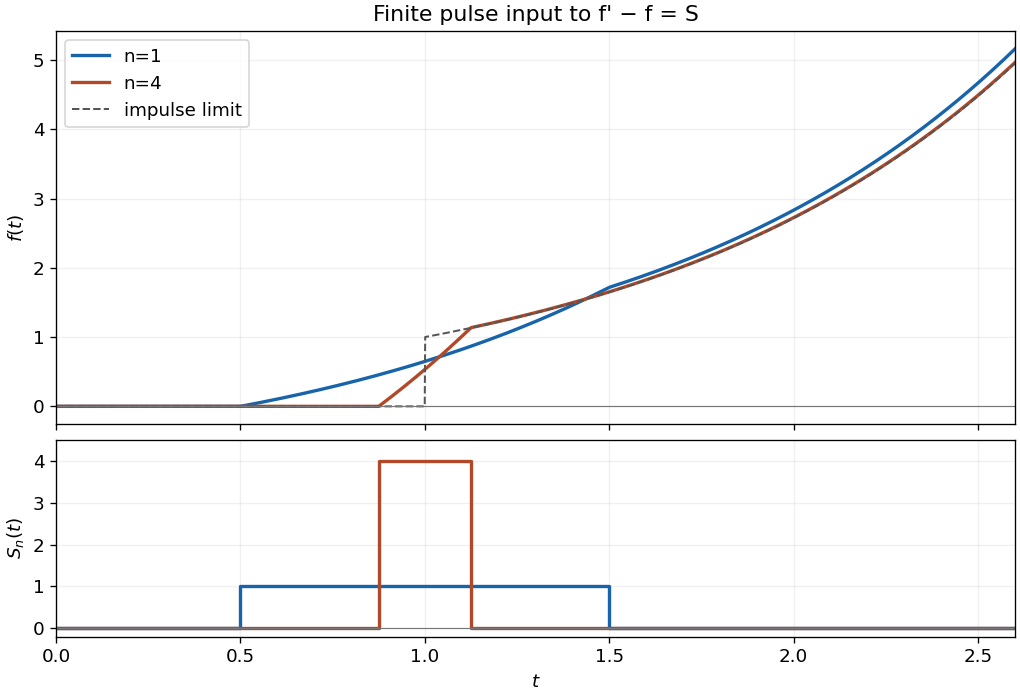
Set $a_n=1-1/(2n)$, $b_n=1+1/(2n)$. The finite pulse has Laplace transform ${\bar{S}}_n(p)=n(e^{-p{a}_n}-e^{-p{b}_n})/p$. Since $f(0)=0$, transforming the equation givesThe partial fraction decomposition $1/[p(p-1)]=1/(p-1)-1/p$ has inverse $e^t-1$. By the Laplace transform time-shift rule,This finite-pulse response of a first-order linear equation gives the requested outer regions:For completeness, while the pulse is active the solution is $n(e^{t-a_n}-1)$. It is continuous at both switching times. After the forcing stops it grows as $e^t$, because the homogeneous equation is $f^{\prime }=f$. The apparent pole at $p=0$ in the full transform is removable; the Bromwich contour may be taken with $c>1$.

Since $P_0=1$, part (d) gives $Q_0^{\prime }=A_0/(1-x^2)$. A partial fraction decomposition and integration give, for $-1<x<1$,The condition at zero fixes $B=0$. Thus the full conclusion from the stated condition isThat condition alone does not fix the multiplicative constant. With the usual Legendre function of the second kind normalization $Q_0^{\prime }(0)=1$, one has $A_0=1$. On real exterior intervals replace the logarithm by $\log |(1+x)/(1-x)|$; complex continuation requires a choice of logarithm branch.