Past exam of the astrophysics course of the University of Oxford / 2018 / 4

A spontaneous emission transition has probability per unit time $A_{ji}$ and emits a photon of energy $h{\nu }_{ji}$. For an optically thin gas, its angle-integrated emissivity is $j_{ji}=n_j{A}_{ji}h{\nu }_{ji}$. Electron collisions populate excited levels at rates $n_e{n}_i{q}_{ij}$; they also remove excitation collisionally at rates $n_e{n}_j{q}_{ji}$, returning the energy to the gas rather than producing the line photon. A collisionally excited line is usually emitted by a subsequent spontaneous radiative decay; collisional de-excitation instead quenches it.

The critical density of an atomic transition compares radiative loss from an upper level with its collisional loss. For a two-level model, $n_{\mathrm{crit}}=A_{ji}/q_{ji}$; for several lower or connected levels use the relevant sums. Below this density, excitation is commonly followed by a photon and the line cools the gas. Above it, collisions increasingly suppress radiative emission per excitation and drive the level populations toward Boltzmann ratios.

Optical forbidden emission lines have small $A$ because an electric-dipole transition is forbidden by a selection rule. Metastable levels survive long enough to radiate in dilute ionized nebulae, although collisions quench them in dense gas. Ratios from closely spaced levels with different critical densities are electron-density diagnostics; ratios involving different excitation energies probe the electron temperature through Boltzmann factors. Combining line emissivities with electron density, temperature and an ionization model estimates ionic abundances.

Infrared fine-structure emission lines connect closely spaced sublevels. Their small excitation energies make them useful over temperature ranges where optical excitation is exponentially suppressed, and dust extinction is usually weaker in the far infrared. They are important coolants and density diagnostics in ionized gas, with the choice of ion specifying the ionization zone. Neither an optical nor an infrared ionic abundance automatically equals the total elemental abundance; unobserved ionization stages require an ionization correction.

Use the complete supplied three-level model, including collisions between levels 2 and 3. Put $g_1=4$, $g_2=4$, $g_3=6$, and denote a collisional rate coefficient by $q_{ij}$. Detailed balance givesAt $T_e=10^4\mathrm{K}$, the supplied collision strengths give, in ${\mathrm{m}}^3{\mathrm{s}}^{-1}$,The rounded optical wavelengths set the excitation energies; treating the fine splitting as very small compared with $k_{\mathrm{B}}{T}_e$ changes none of the main conclusions.

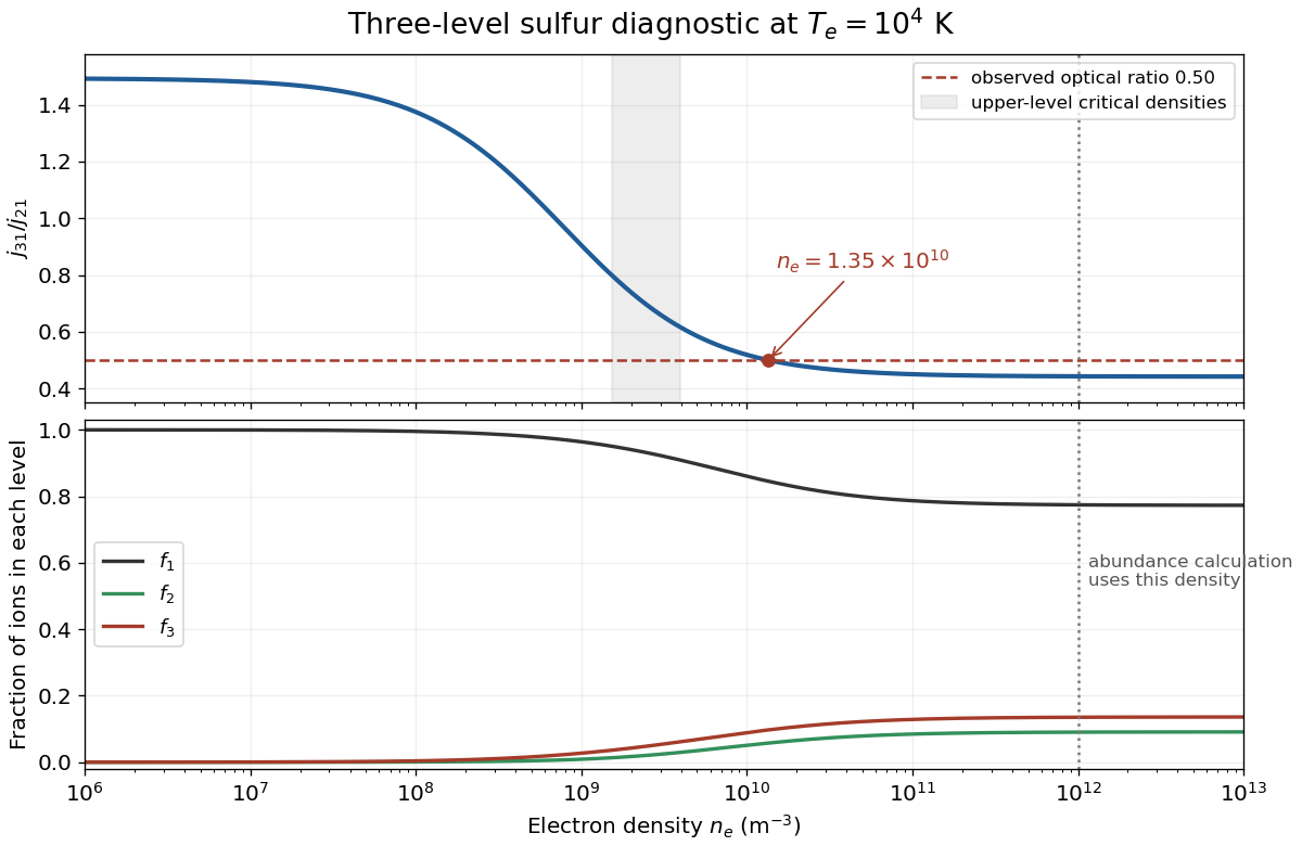
Let $D_2=A_{21}+n_e(q_{21}+q_{23})$, $D_3=A_{31}+A_{32}+n_e(q_{31}+q_{32})$, and $R_{32}=A_{32}+n_e{q}_{32}$. Statistical equilibrium for the upper levels isEliminating $n_1$ yields the line-ratio formulaThe same ratio holds for integrated intensities when the two lines sample the same optically thin volume and differential extinction is negligible. Inserting the data gives the particularly simple numerical formThe low- and high-density limits are approximately $1.49$ and $0.442$. The collisional loss channels giveThus the useful density range is around $10^9$–$10^{10}{\mathrm{m}}^{-3}$. Maximizing $|d\log \mathcal{R}/d\log n_e|$ for the rational expression gives its strongest fractional sensitivity at $n_e=7.8607\times 10^8\sqrt{1.49325/0.442056}=1.44\times 10^9{\mathrm{m}}^{-3}$. Omitting the supplied 3–2 collisions would change the critical densities and inferred density appreciably.

For the observed ratio $0.50$, inversion gives $n_e=1.35\times 10^{10}{\mathrm{m}}^{-3}$. This is on the high-density side of the transition, but is not the infinite-density limit. Solving the statistical-equilibrium equations and imposing $f_1+f_2+f_3=1$ gives the level fractionsA rough high-density estimate would instead use $f_i\propto g_i{e}^{-E_i/(k_{\mathrm{B}}{T}_e)}$; it is useful as a limiting check, not an exact solution for $\mathcal{R}=0.50$.

For the separate abundance calculation, use the expressly prescribed $n_e=10^{12}{\mathrm{m}}^{-3}$. The same model now gives $(f_1,f_2,f_3)=(0.77426,0.09045,0.13528)$, nearly the collisional Boltzmann limit. The measured angle-integrated volume emissivity givesThereforeThis is an abundance per free electron; it is approximately $n({\mathrm{S}}^{+})/n({\mathrm{H}}^{+})$ for predominantly ionized hydrogen with $n_e\simeq n({\mathrm{H}}^{+})$. No $4\pi$ factor is inserted because the supplied emissivity is power per volume, not power per volume per steradian. The imposed $10^{12}{\mathrm{m}}^{-3}$ predicts a ratio about $0.443$, rather than exactly $0.50$; the two numerical instructions cannot both describe one uniform zone exactly within this model.

The source's $2p^3$ configuration label is a typographical error for the sulfur valence configuration $3s^{2}3p^3$. This does not alter the stated $J$ values or the calculation above.^[ref]

The infrared and optical transitions share the same upper level 3. Using the supplied infrared photon energy givesWith the same $T_e,n_e$ and three-level fraction $f_3$ used in the abundance calculation of b,This exceeds the optical abundance by a factor $5.53$. Because the upper level is common, its population cancels in the intrinsic emissivity ratio:The observed ratio is $1.5\times 10^{-5}$. Thus changing only the electron temperature or a common level-population correction cannot reconcile these two lines from the same gas. Dust extinction suppressing the optical line is a natural explanation. If the far-infrared attenuation is negligible, the required optical attenuation isDifferent apertures, filling factors, optical-depth assumptions or emissivity calibrations could also cause a discrepancy. A total sulfur abundance would still need an ionization correction beyond this ionic comparison.