Past exam of the atomic and laser physics course of the University of Oxford / 2022 / 1

In LS coupling, first add the individual orbital angular momenta and spins separately, then add their totals:The Coulomb interaction between electrons must separate different atomic terms more strongly than the spin-orbit interaction mixes them. Then $L,S,J,M_J$ are useful quantum numbers, with $J=|L-S|,\dots ,L+S$. This approximation is usually better for lighter chemical atoms and well-separated atomic terms; strong configuration interaction or strong spin-orbit coupling can spoil it. The term symbol is ${}^{2S+1}{L}_J$.

The general electric-dipole selection rules, for isolated chemical atoms with definite parity and total electronic angular momentum, are a change of parity, $\Delta J=0,\pm 1$ excluding $J=0\leftrightarrow 0$, and $\Delta M_J=0,\pm 1$, with the accessible magnetic sublevels determined by the light's polarization. In pure LS coupling, the additional selection rules are $\Delta S=0$ and $\Delta L=0,\pm 1$, excluding $L=0\leftrightarrow 0$. In a one-electron description the electric dipole operator also requires $\Delta l=\pm 1$ for the active electron. These latter statements can fail as exact labels when atomic terms mix; the general parity and total-angular momentum restrictions still apply. Unresolved hyperfine structure is neglected here.

For strontium, the closed core contributes $L=S=0$. The Pauli exclusion principle makes the two equivalent $5s$ electrons a singlet state. Different radial orbitals permit both a singlet state and a triplet state. Thus the complete lists of atomic fine-structure levels areThe $5s5p$ electron configuration has odd parity; the other two electron configurations have even parity.

Measure each energy level by the wavenumber $\tilde{E}=(E-E_g)/(hc)$ in ${\mathrm{m}}^{-1}$. An upward electronic transition of vacuum wavelength $\lambda$ adds $1/\lambda$. Treat the quoted wavelengths as vacuum values to their limited accuracy; air corrections would be smaller than the precision justified here.

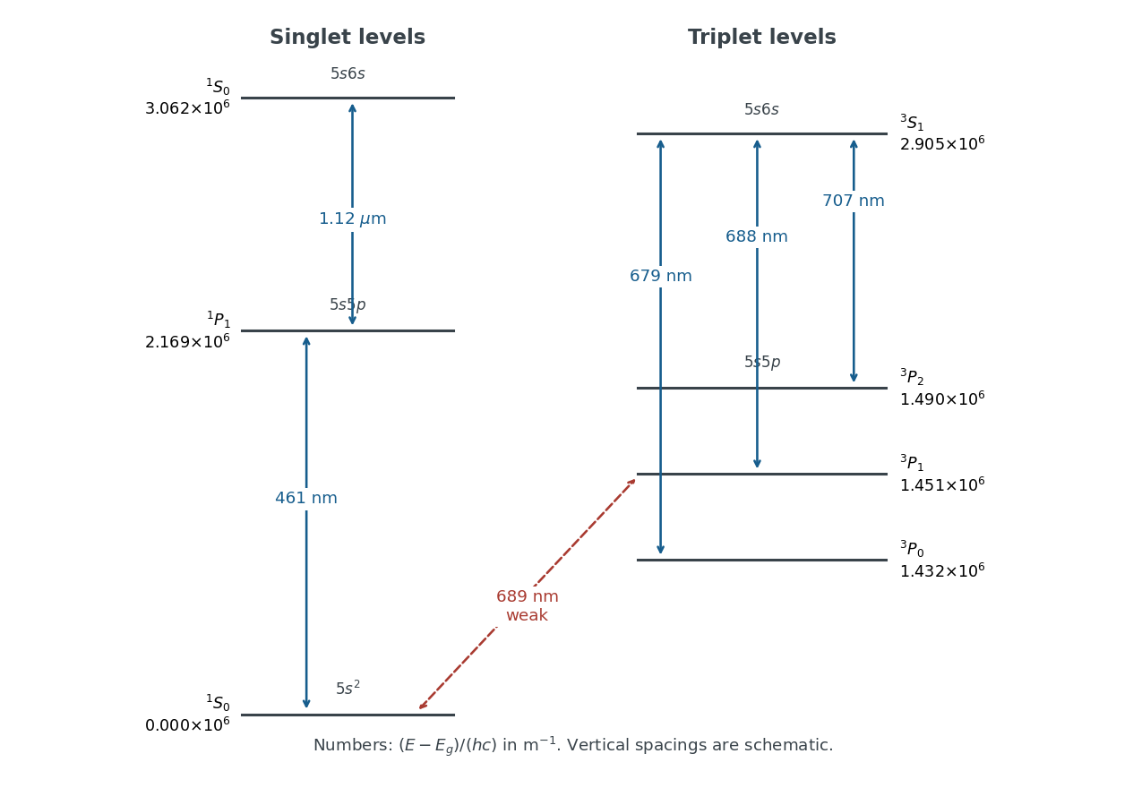
The strong ground-state absorption must be $5s^2{}^1{S}_0\to 5s5p{}^1{P}_1$ at $461\mathrm{nm}$. The weak ground-state electronic transition at $689\mathrm{nm}$ must reach $5s5p{}^3{P}_1$: the electric-dipole selection rule on $J$ excludes the other two triplet state energy levels, while weak spin-orbit coupling admixes singlet state character and relaxes the approximate spin selection rule.

Assume the usual ordering $E({}^3{P}_0)<E({}^3{P}_1)<E({}^3{P}_2)$, as expected from a positive effective spin-orbit coupling constant. The three nearby strong spectral lines then join these energy levels to a common $5s6s{}^3{S}_1$ energy level. Larger lower-state energy means a smaller gap and longer wavelength, so $679,688,707\mathrm{nm}$ correspond to $J=0,1,2$ respectively. The remaining $1.12\mu \mathrm{m}$ spectral line joins $5s5p{}^1{P}_1$ and $5s6s{}^1{S}_0$. Assume the latter is the upper energy level. These assignments and orderings agree with independently tabulated strontium energy levels.^[ref]

Starting with the two ground-state gaps, the construction isThe resulting energy levels, rounded to avoid suggesting spectroscopic precision, are

Both $461\mathrm{nm}$ and $1.12\mu \mathrm{m}$ exhibit the normal Zeeman effect. Each connects two singlet state energy levels, with Landé g-factor $g_J=1$ for the $J=1$ energy level and no first-order shift for $J=0$. Their frequency shifts are $0,\pm {\mu }_{B}B/h$. The weak $689\mathrm{nm}$ spectral line also has three components, but $g({}^3{P}_1)=3/2$ gives shifts $0,\pm 3{\mu }_{B}B/(2h)$; a three-component pattern alone does not establish the normal Zeeman effect. The $679\mathrm{nm}$ spectral line likewise has three components with $g({}^3{S}_1)=2$.

For $5s5d$, addition of angular momentum gives $L=2$ and $S=0,1$. The even-parity atomic terms and atomic fine-structure levels areThe electric-dipole selection rules exclude all connections to the even-parity $5s^2$ and $5s6s$ electron configurations. To the odd-parity $5s5p$ electron configuration, all seven allowed connections in pure LS coupling areHere a connection is listed independently of whether the $5s5d$ energy level is above or below its partner.

In a weak magnetic field, use the Landé g-factorFor the three ${}^3{D}_J$ energy levels, this gives $1/2,7/6,4/3$; for ${}^3{P}_1,{}^3{P}_2$ it gives $3/2$. The six-component spectral line is thereforeA component has frequency displacement $({\mu }_{B}B/h)(m_D/2-3m_P/2)$. The electric dipole transition with $m_D=m_P=0$ has zero matrix element, since the relevant $J=1\leftrightarrow 1$ rank-one Clebsch-Gordan coefficients vanish there. The remaining allowed pairs giveThus all six frequency positions $\pm 1/2,\pm 1,\pm 3/2$ are distinct. Perpendicular to the magnetic field, both the $\pi$ and $\sigma$ components are visible, with mutually perpendicular linear polarizations. Along the magnetic field the $\pi$ components disappear. This is the weak-field Zeeman effect, before the Paschen-Back effect changes the coupling scheme.

The closest components above differ by $\Delta {\nu }_{\min }={\mu }_{B}B/(2h)\simeq 7.0\mathrm{GHz}{\mathrm{T}}^{-1}B$. At $B=0.1\mathrm{T}$, their separation is about $0.70\mathrm{GHz}$. A visible spectral line near $500\mathrm{nm}$ would consequently require spectral resolving power of order $\nu /\Delta {\nu }_{\min }\simeq 9\times 10^5$. An ordinary low-resolution spectrometer would merge the components.

A suitable arrangement places an excited low-pressure strontium discharge or a transversely observed atomic beam between wide electromagnet pole pieces. Collect the emission perpendicular to the magnetic field, select the desired spectral line with a prefilter or monochromator, and send it through a high-finesse scanning Fabry–Pérot interferometer to a detector. A rotatable linear polarizer separates the two $\pi$ components from the four $\sigma$ components. Calibrate both the interferometer's free spectral range and the local magnetic field; take zero-field and several field-strength scans, and fit component positions against $B$.

The magnetic field should be uniform across the viewed volume, with its associated Zeeman splitting larger than the combined natural linewidth, Doppler broadening, pressure broadening and instrumental width, but much smaller than the separations of the relevant atomic fine-structure levels. A collimated transverse atomic beam, low collision rate and restricted collection angle reduce unwanted spectral line broadening. Avoid appreciable power broadening, resolve or model isotope and hyperfine structure, and check for self-absorption. A zero-field scan and the predicted linear scaling help distinguish actual Zeeman splitting components from neighbouring spectral lines.