Use the source's explicit graded production rules. X is already present at a constant concentration; the input at zero activates it rather than starting accumulation of X. Assume its active level exceeds both relevant X thresholds, put , let , and take . Before the input Z is not produced, so use the initial steady value .
For I1 incoherent feed-forward loop, activation of X starts Y production; for I4 incoherent feed-forward loop it stops Y production. ConsequentlyThe two delays are the times for Y to cross its output-regulation threshold. In I1 incoherent feed-forward loop, initially absent Y permits the high output rate, then accumulated Y represses it. In I4 incoherent feed-forward loop, initially abundant Y activates the high output rate, then Y's decay removes that activation. Thus both have production before their respective delay and afterwards.
With and , their common piecewise response, with or , isThe output is continuous at the production switch. There is an overshoot precisely when ; otherwise it rises monotonically to . For a threshold not extremely close to its limiting values and the supplied , a rapid pulse followed by relaxation to a lower nonzero level is expected. This can provide fast initial response or a transient strong signal, but it is not perfect adaptation to the original zero output.
The original plots below use the illustrative values and . At the two Y curves are complementary and their output delays and Z curves are identical. These threshold values are examples, not extra source data. “AND” here must be read with the stipulated graded rates: replacing them by an ordinary all-or-nothing AND rule would give a different response.
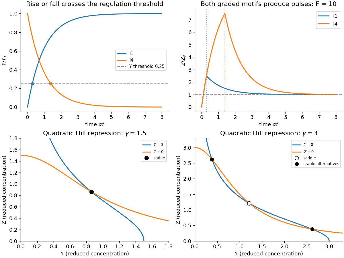
Graded incoherent feed-forward pulses and the change from one to two attracting toggle states
. Original model trajectories and nullclines. Pulse panels use illustrative , and dimensionless time ; switch panels use with the explicitly labelled reduced production strengths. Details.
For the final low steady value , the first crossing of occurs during high production if . Solving then gives, for either motif,This half-final response of a graded incoherent feed-forward loop is a first-crossing measure. A simple output produced at the final low rate from zero would instead take . This comparison explains the acceleration of the first half-final response, not the time needed to settle after a potentially large overshoot.
The condition matters because the source does not fix . Define , equal to for I1 incoherent feed-forward loop and for I4 incoherent feed-forward loop. If the high phase ends before half-final output is reached, solve the second branch of part (a) instead:The expressions agree at the boundary. The -only answer is therefore valid for both motifs when , as holds for large F and a fixed interior threshold. Merely saying does not cover a threshold that approaches zero or one even faster. If the Y threshold is never crossed, the assumed final low state itself changes and one must reconsider the steady state before using this response-time definition.
At the final steady state, the ligands control activity as well as the amount of each factor. Assuming active X exceeds its thresholds and the high Y level exceeds , the normalized output production rates areFor I1 incoherent feed-forward loop, active X makes Y abundant, but Y can repress Z only if its own activating ligand is present. Without , Y is inactive and the output remains high. For I4 incoherent feed-forward loop, active X represses Y to below its threshold, so the output is low regardless of . If X is inactive, the direct permissive arm is absent and both outputs are zero even when Y is active.
Thus I1 incoherent feed-forward loop can retain two-input combinatorial control at steady state as well as generate the transient in part (a). I4 incoherent feed-forward loop loses steady-state sensitivity to once X has suppressed Y, under these particular assumptions. That gives a functional reason the first motif may be more useful in many regulatory contexts. It is not a proof of an evolutionary frequency: promoter implementation, thresholds, noise, costs and other functions also influence how common a motif is. The argument follows the supplied rate table, including its nonzero , rather than a generic Boolean AND truth table.
Use Y and Z as the variables appearing in the equations; the introductory reference to X and Y is a naming mismatch. With , , a symmetric equilibrium has andThe left side increases continuously from zero to infinity because its derivative is . Thus there is exactly one positive symmetric solution for every allowed parameter pair, which verifies the implicit steady-state expression.
For and , look for one high component and one low component. If , the other equation gives ; that small value in turn gives . Exchanging the components gives the alternative state:For example the relative correction to the high value is of order , while the low value first has the ordinary denominator correction of relative order . The sharply repressive Hill function is therefore consistent with two alternatives, one factor high and the other low, which can encode a switch. Mutual repression makes a positive feedback loop: a high Y suppresses Z and thereby relieves repression of Y. Existence of alternative equilibria alone does not establish their stability; the explicit quadratic-Hill case in part (e) also permits that check.
The quadratic-Hill mutual repression switch is explicit: for , steady state requires and . Subtraction givesThus either , giving the unique positive cubic root , or . In the latter case, , henceThe non-symmetric pair is real, positive and distinct exactly when . For only the symmetric solution exists. Eliminating one variable gives the source's hinted factorization,with no singular denominator for real concentrations. The cubic is strictly increasing since , so it contributes only the symmetric state.
One can verify the switch interpretation without a lengthy stability analysis. At symmetry the Jacobian matrix eigenvalues are : symmetry is stable for and becomes a saddle for , corresponding to and . At either asymmetric equilibrium the eigenvalues are , both negative when . ThereforeAt , all three branches meet at with a zero linear eigenvalue, the switching threshold rather than two distinct robust memory states. The lower panels of the original figure in solution show representative nullclines on either side.
Articles by others on the same topic
There are currently no matching articles.