For the driven two-state rotary motor, use positive angular velocity and extend all angular functions with period . In the first half-turn the source figure has , , so the stationary equation is . In the second half-turn the rates are interchanged, giving . HenceContinuity at gives , while periodicity gives . Solving the two linear conditions gives andIn particular and , so the two pieces fill in the apparent endpoint gap in the printed piecewise formula. The probability decreases exponentially during the detachment half-cycle and rises exponentially during the attachment half-cycle; is its complement. Both remain between zero and one. They are state probabilities conditional on rotor angle, not separate angular densities normalized individually to one.
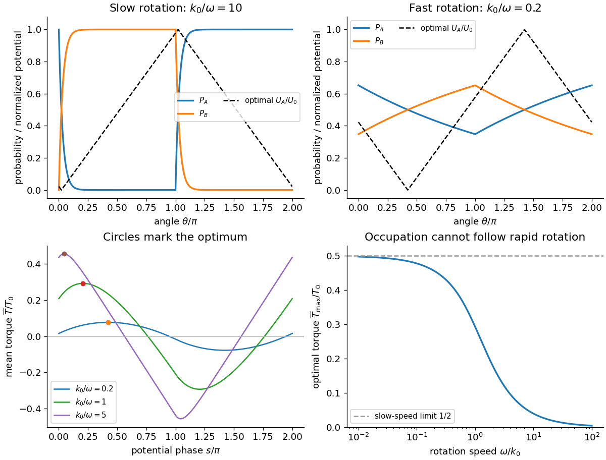
For , attachment and detachment almost finish within their allotted half-turns: is nearly zero through most of and nearly one through most of , with angular boundary layers of width . For , it stays near one half with a small nearly triangular modulation. The upper panels of the original figure in part (b) sketch both limits. At exactly zero speed the advective stationary problem is singular; these statements concern the positive-speed limit.
The source potential rises from zero to over the half-turn from to , then falls over the next half-turn. Its slopes are . Torque is minus the angular derivative of potential; in the detached state is angle-independent and exerts no torque. A uniform set of motor phases therefore givesHere is an energy and a torque because the angle is in radians. The average over a full turn divides by , rather than by the bound-state occupation alone.
Differentiating the moving integration limits and using periodicity givesThe optimal phase of a two-state rotary motor follows on : decreases, so the stationary point is a maximum and satisfiesThe crossing displaced by is the corresponding minimum. For slow positive rotation, lies just after the detachment switch. The potential then rises mainly while the motor is detached and falls mainly while it is bound. For fast rotation, , with only a small phase-dependent occupation available to produce torque. The potential should still be shifted by this optimum, rather than aligned arbitrarily with a rate switch.
The half-turn symmetry gives . At the optimum, direct integration of the two exponential pieces gives . Thus a useful exact check isFor fast rotation, instead tends to zero. The original plots below show the calculated probabilities and optimized potential shapes. The imposed switching rates constitute driven kinetics: their strictly one-way windows are not equilibrium detailed balance at a fixed angle. Sustained work requires the motor's chemical/ion-gradient energy supply, not extraction of work from a passive single thermal bath.

The AFM pulls a tethered molecule through its cantilever. Deflection, multiplied by a calibrated cantilever spring constant, measures force; support motion must be corrected for that deflection and any linker compliance to obtain molecular extension. Initially folded structure can resist extension, then contacts break and more polypeptide polymer contour length becomes available. The readable trace rises with increasing extension, with fluctuations and a strongly rising large-extension part. It should not be interpreted as a direct image of individual amino acids or as establishing a unique microscopic unfolding pathway.
An ideal inextensible freely jointed chain with the stated segment count and length hasIts mean extension is strictly below at every finite force. Thus the quoted maximum does not establish ideal FJC behaviour: if both numbers are taken literally, it exceeds the model's polymer contour length by about . Finite segment stretch, inaccurate effective segment parameters, additional linkers or an extension-zero/calibration error can account for such a difference. If the numerical descriptions are approximate, the discrepancy may be within their uncertainty; even exact agreement with a polymer contour length would not prove freely jointed statistics. Low-force fluctuations and the full force–extension relation are separate tests.
Let a segment of fixed length make angle with an applied force . Its energy contribution is . Independent freely jointed orientations give the single-segment partition function and chain partition functionThe mean end-to-end projection is the force derivative of :For , the Langevin function is . Isotropy therefore gives the vector responseThe covariance at zero force provides an independent route: , and the Boltzmann weight's first-order term yields . This is a relation for the mean vector or its projection. The zero-force mean vector vanishes even though the chain has finite root mean square size .
The controlled weak-force condition is , not merely that a short part of a measured curve looks straight. With the supplied , at . A raw force near , as in the figure's labelled low-extension portion, would give and is not asymptotically weak for those literal segment parameters. A force offset or different effective model might change that interpretation, but no such correction should be invented from the plot.
The coefficient in the linear force law isStretching suppresses the many disordered orientations available to the chain. The Gaussian chain free energy cost has gradient equal to this restoring force. This is entropic elasticity; individual covalent bonds need not stretch to produce the weak-force spring.
At moderate force, even an ideal FJC becomes nonlinear as its orientations align, so failure of a linear fit alone need not imply nonideal chemistry. But failure of the full FJC curve can reflect backbone spring constant and correlated segment angles, nonuniform effective links, remaining folded contacts, force-induced conformational changes, energetic bond compliance, or tether/calibration effects. An extensible FJC or an appropriate semiflexible model includes some of these effects; their parameters require independent justification. The stated inextensible polymer contour length already excludes a literal extension.
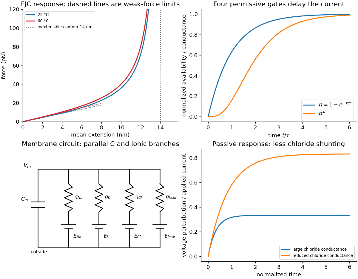
The first panel of the original model figure below shows the full orientational response and weak-force tangents without tracing the experimental data.

If the ideal-chain segment count and segment length remain fixed, the entropic spring constant is proportional to absolute temperature. ThereforeThis is an increase by about . The factor multiplies the free energy penalty for the loss of chain configurations; a larger force is required to impose the same normalized weak extension at higher temperature.
Not degrading does not guarantee that a real protein's folded state, effective spring constant or solvent interactions remain unchanged. Thermal unfolding and changes in persistence length can occur without covalent degradation. Those changes modify the experimental curve and may invalidate a fixed- comparison. The boxed value is the explicit ideal-FJC prediction under fixed segment geometry, not an unconditional thermal-stability prediction for the protein.
On releasing the tensile load, the extended chain first retracts towards less aligned conformations because they have much greater configurational multiplicity. Viscous friction and internal relaxation determine the time course; stored free energy is dissipated as heat. An unconstrained ideal chain does not shrink to a point: its mean vector is zero but its root mean square end-to-end length is for the supplied ideal-chain parameters.
A real polypeptide also has sequence-dependent interactions. If the original native structure is the stable state in the prevailing solvent and the molecule remains intact and capable of folding, it can subsequently refold, gaining favourable intramolecular and solvent free energy. The folded state is not selected by chain entropy alone, and formation of native contacts need not be instantaneous. Kinetic traps, proline isomerization, protein aggregation, misfolding, surface attachments or chemical damage may prevent complete recovery or produce hysteresis. Thus reversible refolding is a physically motivated possibility, not guaranteed simply by removal of force. This distinction connects the recoil of a stretched polymer to the thermodynamics discussed in Question 6(c).
Represent one permissive voltage-gated potassium channel gate by an available closed state and an activated state, with voltage-dependent transition rates and . Gain minus loss givesDuring a voltage clamp step the imposed voltage and hence these rates are constant. Integration with givesThe fourth power in the electrical conductance describes four permissive activation variables in the Hodgkin-Huxley model phenomenology. If all must be permissive and are statistically independent, their joint probability is . Even a simple exponential rise in then gives a delayed-looking macroscopic potassium electric current. The second panel of the model figure in solution illustrates this. A continuously changing voltage makes the rates time dependent and requires solving the differential equation along that voltage trajectory; one fixed exponential is not the general action-potential solution.
selective permeability sets the driving-force term. Potassium and sodium channels provide narrow coordinating pathways whose free energy balance of hydration and chemical binding favours the appropriate ion. voltage-gated potassium channel carbonyl coordination differs from the charged filter environment in canonical sodium channels, so selective permeation is not a pore-size ranking. Ion substitution shifts the reversal potential, and selective blockers or filter mutations alter the corresponding electric current. An open channel conducts down the electrochemical gradient; ATP-driven pumps maintain the gradients rather than pushing each ion through the pore.
Voltage-dependent activation sets channel availability. Charged residues in the S4-containing voltage-sensing domains move in the membrane electric field and couple to pore opening. A classical voltage-gated potassium channel is a tetramer; a voltage-gated sodium channel pore-forming polypeptide has four homologous domains. ion-channel gating current measurements and sensor-residue mutations connect electric charge motion to opening, while structures separate the sensor from the permeation pathway. The historical and variables describe kinetics phenomenologically and need not map one-to-one onto individual resolved structural movements.[ref]
Voltage-sensing residues in the S2 and S4 segments of the Shaker K+ channel by S. A. Seoh and others. Sensor perturbations and measured gating charge
[ref]Time dependence, especially ion-channel inactivation, explains the different electric current waveforms. Sodium activation is rapid, but sustained depolarization reduces the availability variable , so the sodium electric current decays despite maintained driving voltage. Fast sodium ion-channel inactivation involves intracellular machinery including the interdomain III–IV region. Potassium activation is slower, supplying delayed outward electric current; the classical delayed rectifier is relatively sustained on this time scale. Some voltage-gated potassium channel variants do show rapid N-terminal pore-blocking ion-channel inactivation or slower filter-associated ion-channel inactivation, which should not be assumed identical to sodium's mechanism. voltage clamp steps separate activation from decay; recovery protocols, single-channel recordings and targeted perturbations distinguish gating, ion-channel inactivation and ion conduction. Removal of the Shaker N-terminal blocker and restoration by a free peptide are particularly direct evidence for one voltage-gated potassium channel mechanism.[ref]
Biophysical and molecular mechanisms of Shaker potassium channel inactivation by Toshinori Hoshi and others. N-terminal perturbations separate rapid inactivation from activation
[ref]Restoration of inactivation in mutants of Shaker potassium channels by a peptide derived from ShB by William N. Zagotta and others. Cytoplasmic peptide restores the missing blocking process
Together these properties produce and : selectivity fixes reversal potential, maximal electrical conductance fixes scale, and activation/inactivation variables supply voltage- and history-dependent open probability.
Including both end faces of the perfect cylinder, with and ,The membrane capacitance is . The required net inward electric charge is , or monovalent ions. If sodium supplies that net electric charge, Faraday constant givesThe final concentration is about , only above the starting value. Neglecting the end faces changes the estimate by , giving about . Over the capacitive electric charge corresponds to mean net electric current ; the duration does not otherwise enter the total electric charge.
This is a net capacitive estimate, not a measurement of total sodium influx. Simultaneous outward potassium electric current makes actual sodium entry larger, and most bulk ions remain near their original concentrations during one spike. Long-term pumps restore gradients after repeated firing; they are not required to replace the entire intracellular sodium pool during the two-millisecond voltage rise.
The equivalent circuit has membrane capacitance in parallel with electrical conductance–battery branches: voltage-dependent sodium and potassium conductances in series with their reversal potentials, a chloride electrical conductance in series with , and other leak conductances. For externally supplied electric current,The model figure in solution includes this circuit and an illustrative passive response. Although chloride electric current is small when , a perturbation produces the restoring electric current . A large chloride electrical conductance therefore shunts perturbations, lowers input resistance and shortens the passive time constant, and .
Reducing that electrical conductance increases the voltage response to a given electric current or extracellular-potassium disturbance and weakens stabilization near rest, making repeated excitation easier. There need not be an instantaneous shift of resting voltage if equals the old rest exactly. In skeletal muscle, loss of ClC-1-mediated stabilization is associated with myotonic hyperexcitability.[ref]
The skeletal muscle chloride channel in dominant and recessive human myotonia by Manuela C. Koch and others. Channel defects associated with inherited muscle hyperexcitability
Later cessation of contraction can be explained by sustained depolarization causing voltage-gated sodium channel ion-channel inactivation and failure to recover: fewer available channels support progressively smaller or less frequent spikes until depolarization block occurs. Accumulated extracellular potassium in restricted spaces and incomplete recovery between spikes can promote that depolarization. This requires the nonlinear voltage-gating dynamics; a passive chloride resistor and capacitor alone cannot generate or terminate an action-potential train. The stated membrane permeability change does not uniquely determine the time to block or prove one particular ionic accumulation history.
Use the source's explicit graded production rules. X is already present at a constant concentration; the input at zero activates it rather than starting accumulation of X. Assume its active level exceeds both relevant X thresholds, put , let , and take . Before the input Z is not produced, so use the initial steady value .
For I1 incoherent feed-forward loop, activation of X starts Y production; for I4 incoherent feed-forward loop it stops Y production. ConsequentlyThe two delays are the times for Y to cross its output-regulation threshold. In I1 incoherent feed-forward loop, initially absent Y permits the high output rate, then accumulated Y represses it. In I4 incoherent feed-forward loop, initially abundant Y activates the high output rate, then Y's decay removes that activation. Thus both have production before their respective delay and afterwards.
With and , their common piecewise response, with or , isThe output is continuous at the production switch. There is an overshoot precisely when ; otherwise it rises monotonically to . For a threshold not extremely close to its limiting values and the supplied , a rapid pulse followed by relaxation to a lower nonzero level is expected. This can provide fast initial response or a transient strong signal, but it is not perfect adaptation to the original zero output.
The original plots below use the illustrative values and . At the two Y curves are complementary and their output delays and Z curves are identical. These threshold values are examples, not extra source data. “AND” here must be read with the stipulated graded rates: replacing them by an ordinary all-or-nothing AND rule would give a different response.
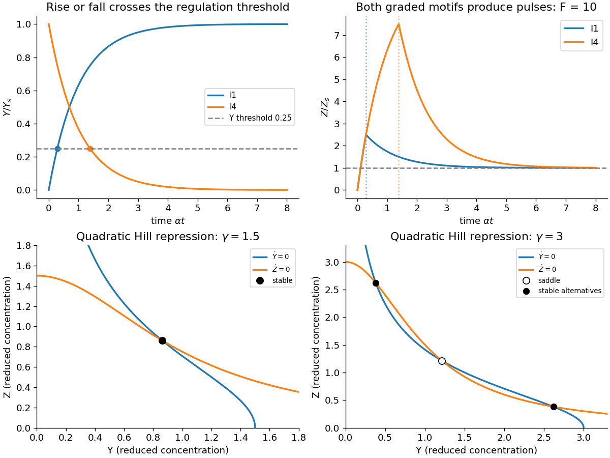
Graded incoherent feed-forward pulses and the change from one to two attracting toggle states
. Original model trajectories and nullclines. Pulse panels use illustrative , and dimensionless time ; switch panels use with the explicitly labelled reduced production strengths. Details.
For the final low steady value , the first crossing of occurs during high production if . Solving then gives, for either motif,This half-final response of a graded incoherent feed-forward loop is a first-crossing measure. A simple output produced at the final low rate from zero would instead take . This comparison explains the acceleration of the first half-final response, not the time needed to settle after a potentially large overshoot.
The condition matters because the source does not fix . Define , equal to for I1 incoherent feed-forward loop and for I4 incoherent feed-forward loop. If the high phase ends before half-final output is reached, solve the second branch of part (a) instead:The expressions agree at the boundary. The -only answer is therefore valid for both motifs when , as holds for large F and a fixed interior threshold. Merely saying does not cover a threshold that approaches zero or one even faster. If the Y threshold is never crossed, the assumed final low state itself changes and one must reconsider the steady state before using this response-time definition.
At the final steady state, the ligands control activity as well as the amount of each factor. Assuming active X exceeds its thresholds and the high Y level exceeds , the normalized output production rates areFor I1 incoherent feed-forward loop, active X makes Y abundant, but Y can repress Z only if its own activating ligand is present. Without , Y is inactive and the output remains high. For I4 incoherent feed-forward loop, active X represses Y to below its threshold, so the output is low regardless of . If X is inactive, the direct permissive arm is absent and both outputs are zero even when Y is active.
Thus I1 incoherent feed-forward loop can retain two-input combinatorial control at steady state as well as generate the transient in part (a). I4 incoherent feed-forward loop loses steady-state sensitivity to once X has suppressed Y, under these particular assumptions. That gives a functional reason the first motif may be more useful in many regulatory contexts. It is not a proof of an evolutionary frequency: promoter implementation, thresholds, noise, costs and other functions also influence how common a motif is. The argument follows the supplied rate table, including its nonzero , rather than a generic Boolean AND truth table.
Use Y and Z as the variables appearing in the equations; the introductory reference to X and Y is a naming mismatch. With , , a symmetric equilibrium has andThe left side increases continuously from zero to infinity because its derivative is . Thus there is exactly one positive symmetric solution for every allowed parameter pair, which verifies the implicit steady-state expression.
For and , look for one high component and one low component. If , the other equation gives ; that small value in turn gives . Exchanging the components gives the alternative state:For example the relative correction to the high value is of order , while the low value first has the ordinary denominator correction of relative order . The sharply repressive Hill function is therefore consistent with two alternatives, one factor high and the other low, which can encode a switch. Mutual repression makes a positive feedback loop: a high Y suppresses Z and thereby relieves repression of Y. Existence of alternative equilibria alone does not establish their stability; the explicit quadratic-Hill case in part (e) also permits that check.
The quadratic-Hill mutual repression switch is explicit: for , steady state requires and . Subtraction givesThus either , giving the unique positive cubic root , or . In the latter case, , henceThe non-symmetric pair is real, positive and distinct exactly when . For only the symmetric solution exists. Eliminating one variable gives the source's hinted factorization,with no singular denominator for real concentrations. The cubic is strictly increasing since , so it contributes only the symmetric state.
One can verify the switch interpretation without a lengthy stability analysis. At symmetry the Jacobian matrix eigenvalues are : symmetry is stable for and becomes a saddle for , corresponding to and . At either asymmetric equilibrium the eigenvalues are , both negative when . ThereforeAt , all three branches meet at with a zero linear eigenvalue, the switching threshold rather than two distinct robust memory states. The lower panels of the original figure in solution show representative nullclines on either side.
In a bacterial transcription complex, RNA polymerase binds a promoter and locally separates the DNA strands into a transcription bubble. The template enters the active site in the to direction, while the complementary RNA grows to . The displaced non-template strand passes around the bubble, downstream DNA re-forms a duplex, and the nascent RNA exits through a separate channel. A short RNA–DNA hybrid is maintained in an elongating complex; the first few nucleotides of an initiating complex do not yet make a full elongation-length hybrid.
The core enzyme has subunit composition ; association with a sigma factor forms a promoter-selective holoenzyme. Sigma recognizes promoter features and assists steps leading from a closed bound complex to the open complex. Different sigma factors redirect transcription towards different promoter classes. The familiar and elements are examples for a major bacterial sigma family, not a universal sequence rule for all sigma factors. Promoter escape changes these contacts, but complete sigma dissociation at one exact transcript length should not be assumed for every complex.
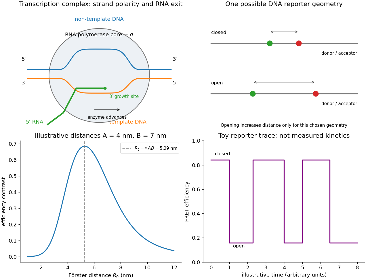
For the supplied non-template sequence, assuming its first base is the first transcribed position, the complementary template runs -TCAGTAAGC-. The RNA has the coding-strand order with uracil replacing thymine. Therefore the first five nucleotides areThe top-left panel of the original schematic in part (d) shows the strand polarities and polymerase organisation; it is not a copied experimental illustration.
The single-block DNA zipper partition function retains one contiguous paired block and ignores multiple separated bubbles. A block of paired bases can start at any of positions. Its first pair has initiation weight , and the remaining pairs each have propagation weight . ThusThe source's symbol in the displayed expressions denotes the same initiation constant as , not Boltzmann's constant. Association and other reference-state factors are absorbed into that statistical weight; the model treats the propagation weights as uniform despite the actual sequence's different bases.
Put . Since counts how many terms of a finite geometric series contain ,ConsequentlyThe apparent singularity is removable: at , the original sum gives , which is for these nine bases.
At , the longest block dominates:Conditional on at least one pair, the fully paired probability approaches one, with leading correction of order . If a fully unpaired reference state of weight one is included, the full partition function is , so a large propagation constant alone does not guarantee predominant duplex if is still very small.
The given sequence contains five A–T and four G–C pairs when fully complementary. Real duplex stability also depends strongly on stacking, sequence context, salt and temperature; it cannot be calculated just by counting two versus three hydrogen bonds. All else comparable, sequences with greater duplex propagation stability resist bubble opening more strongly, while easier-to-open, often A–T-rich start-site regions facilitate initiation. The homogeneous- zipper demonstrates that principle but does not resolve a quantitative sequence-specific melting profile or polymerase's active stabilization of the open state.
To find the optimal Förster distance for two-state contrast, take positive distinct distances and put . The magnitude of the efficiency change isIts derivative has the sign of . It rises from zero, has a single maximum at , then falls back to zero. HenceThe printed form is equivalent, sinceAt this optimum the two efficiencies sum to one and the maximal contrast is . If , there is no distance change and the contrast is zero for every ; the source's unsimplified expression is then and does not specify a unique optimum. For example yields zero contrast regardless of the fluorophore pair. The geometrical-mean result is a design criterion for distinct distances within the assumed fixed-orientation/photophysics FRET law, not a correction for dye-orientation changes.
Place a FRET donor and FRET acceptor on DNA positions whose separation reports start-site opening, using an independently calibrated closed/open geometry and a pair whose Förster distance is near the geometric mean from part (c). Opening may increase or decrease the measured separation depending on where the dyes are placed; anticorrelated donor/acceptor changes need structural and photophysical controls before being assigned to bubble formation.
Single molecules can be observed by low-background fluorescence microscopy while recording FRET donor and sensitized FRET acceptor photons. Correct background, spectral leakage, direct FRET acceptor excitation and unequal detection/quantum-yield factors before calculating efficiency, for example with the corrected intensities. Alternating excitation or independent FRET acceptor observation checks that a low-FRET interval is not simply a dark or bleached FRET acceptor. Intensity anticorrelation, FRET donor lifetime and suitable inactive/closed-state controls strengthen the assignment. The original figure below separates the mechanistic schematic from a purely illustrative model trace.
For the binding-plus-opening first-passage time, a minimal kinetic scheme is , for unbound, closed bound and open bound states. A binding rate , dissociation rate and opening rate already produce multiple waiting-time contributions. With O treated as absorbing during the measurement and starting from U, the mean first-opening time isnot simply . This follows from and . A bound-state marker, or measurements over concentration and a justified kinetic model, helps distinguish binding from opening when unbound and closed DNA share a FRET level.
Fit transitions and dwell distributions with finite time resolution, missed short states, bleaching and censoring included. An open-state exponential dwell can estimate its exit rate under a simple Markov model, while competing closing and dissociation channels require separate observables or additional assumptions. Starting from a defined bound closed state can isolate opening more directly, but dissociation still competes if appreciable. Resolving repeated opening and closing gives forward and reverse kinetics; irreversibility should only be assumed over a demonstrated observation window. The experiment measures a conformational reporter, so a two-level trace alone does not uniquely prove every microscopic step of open-complex formation.

PALM separates emitters in time. A sparse subset of photoactivatable or photoconvertible labels is switched on so that its diffraction-broadened images can be fitted individually; repeated activation, imaging and localization builds a map from many isolated detections. The positional uncertainty can be much smaller than the point spread function width because many photons estimate one image centre: ideally for image width and detected photon number .
That is fluorescence localization precision, not automatically the structural resolution of the reconstructed cell. Pixelation, background, imperfect optics, drift, label linkage, blinking and labelling density matter. Repeated localizations of one molecule cannot fill unlabelled gaps; a crowded frame with overlapping images cannot simply be treated as many isolated emitters. For a static structural map, the structure must remain sufficiently stable while the many frames are accumulated, or its time dependence must be reconstructed explicitly.
For mobility in living cells, keep activated proteins observable for successive frames and link isolated positions into trajectories before bleaching. Repeating this for successive sparse subsets yields many trajectories without making the entire protein population simultaneously fluorescent. This is the sptPALM strategy.[ref]
For free isotropic two-dimensional diffusion with per-coordinate localization error and instantaneous exposures,Fit several lags or a full trajectory likelihood to infer D and its uncertainty. Finite exposure causes motion blur; for a uniform shutter of duration , a simple correction is . Confinement, directed motion and switching binding states change the lag dependence. Short tracks, missed detections and false linking in crowded regions can mimic apparent heterogeneity, so mobility classes require explicit measurement-error and tracking controls. A trajectory map recovers dynamics; it is not identical to a static PALM density map.
The RNA world hypothesis proposes an early stage in which RNA-like molecules carried heritable sequence information and also performed important catalytic functions, before the present division of labour among DNA, RNA and proteins. Complementary base pairing supplies a route to template-directed information copying, while sequence-dependent RNA folding can create catalytic structures. This helps address the apparent circularity of requiring protein enzymes to copy genes whose expression already requires an elaborate protein-synthesis apparatus.
Modern biology supplies evidence for the necessary capacities. Ribozymes catalyse reactions, and self-splicing introns demonstrate RNA-dependent processing without a dedicated protein enzyme for that chemistry. The ribosome's peptidyl-transferase centre is built principally from RNA, with catalytic geometry located in its RNA core; structural work provides direct evidence that this central protein-synthesis chemistry is RNA based.[ref]
The structural basis of ribosome activity in peptide bond synthesis by Poul Nissen and others. Structures and substrate-analogue complexes identify an RNA-based peptidyl-transferase active site
RNA also remains central as messenger, adaptor and regulatory material. These observations make RNA catalysis and information storage physically plausible rather than assuming that all catalysts must be proteins.They do not prove a complete historical sequence. A viable early system still needs plausible nucleotide supply and activation, polymerization, template copying with sufficient fidelity, product-strand separation, compatibility of catalytic and copying conditions, an energy source and some means of maintaining useful combinations. RNA's chemical lability and the challenge of separating paired products are constraints, not details supplied automatically by base pairing. The first hereditary chemistry might also have involved related polymers or cooperative RNA–peptide systems rather than an exclusively RNA organism.
The later advantages of DNA as a relatively stable storage medium and proteins as catalysts with chemically varied side chains help explain the present division of labour. The hypothesis is therefore a testable family of evolutionary scenarios supported by molecular capabilities and biological relics, not a direct observation of prebiotic life or proof that an isolated modern RNA already self-replicates autonomously.
A stable native conformation is favoured when its Gibbs free energy, including the protein and its surrounding solvent, is lower than that of competing conformational ensembles under the specified conditions:Folding greatly reduces the chain's conformational entropy, an unfavourable contribution. It can nevertheless gain favourable hydrogen-bonding and packing interactions, van der Waals contacts, screened electrostatic interactions and solvent free energy. In aqueous globular proteins, burying nonpolar surface reduces the cost of exposing it to water; the hydrophobic effect is not an extra covalent attraction between all hydrophobic residues. Hydrogen bonds and ionic contacts must be judged relative to the interactions those groups made with solvent before folding, so merely counting bonds in the folded structure does not determine stability.
The protein primary structure determines which contacts and protein secondary structures can cooperate. A free-energy landscape biased towards compatible contacts permits many routes towards the native ensemble, rather than an exhaustive random search through every conformation. Folding funnels describe this bias, while barriers explain metastability and folding rates. Reversible denaturation/refolding experiments show that some proteins can recover native structure and activity when suitable conditions are restored, supporting a sequence-encoded thermodynamic tendency without asserting that every protein folds unaided.
“Stable” means an equilibrium preference and a useful lifetime, not one perfectly rigid shape. Native proteins fluctuate and can have several functional conformations; the unfolded ensemble remains populated with relative weight depending on its full free energy. Changes of temperature, pH, salt, solvent, ligands or pressure alter the balance, and molecular chaperones can prevent protein aggregation or assist kinetic access without supplying a different primary sequence. Membrane proteins require their appropriate environment, and intrinsically disordered proteins need not possess one stable folded state in isolation.
Thus a released stretched chain can gain configurational entropy on first recoiling yet later favour a more ordered native structure because the total free energy balance, including solvent, is different. Equilibrium stability, barriers to unfolding and resistance to irreversible protein aggregation are distinct properties. The existence of a native minimum alone does not guarantee rapid, reversible folding under every experimental condition.
Articles by others on the same topic
There are currently no matching articles.