Past exam of the computer science course of the University of Oxford / 2021 / Artificial intelligence / 1

All three variants are complete search algorithms under the usual finite-branching factor, nonnegative-heuristic function assumptions. Here $0\le h\le h^{\ast }$, with zero at goals; the supplied positive lower bound on step costs is also essential. The root is processed once before a parent-dependent priority is needed.^[ref] Completeness means finding a solution if one exists, not necessarily terminating when none exists.

Fix a finite solution path. Every search node on that path has a finite priority, so let $K$ bound all of its relevant priorities. For ordinary A-star search and the second variant, the priority is at least $g(n)$. Thus any search node with priority at most $K$ has depth at most $\lfloor K/ϵ\rfloor$. In the third variant the priority is at least $g(n^{\prime })$, so its depth is at most $\lfloor K/ϵ\rfloor +1$. A finitely branching search tree has finitely many search nodes at these depths. Therefore finitely many earlier search nodes can delay each successive search node on the chosen solution path; eventually its goal is generated or selected, as appropriate.

Moving the goal test to generation cannot destroy that existence guarantee, although it can destroy optimality. Likewise the altered parent-dependent priorities remain bounded below by the accumulated cost to the search node or its parent, which is enough for this completeness argument. If “admissible” were interpreted to allow arbitrarily negative estimates, the lower-bound argument would need an additional hypothesis; the conventional nonnegative interpretation is being used explicitly. For the literal upper-bound-only interpretation, all three can fail completeness: attach an infinite unit-cost dead-end chain with $g(n_d)=d$ and $h(n_d)=-2d$ beside a finite goal branch beginning with a cost-$3$ edge and estimate zero. Its successive low priorities can starve the finite branch. Every negative chain estimate is still at most its infinite true remaining cost.

None of the three variants is an optimal search algorithm in general. The following single search tree supplies counterexamples for all three. Its heuristic function is nonnegative, admissible and even a consistent heuristic.

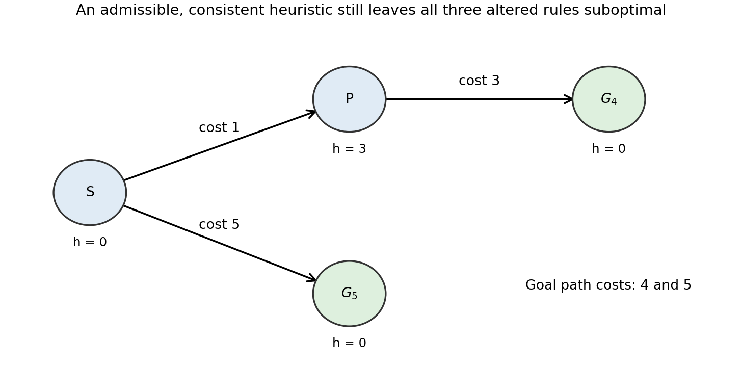
The least-cost goal is $G_4$, reached at cost $1+3=4$; the other goal $G_5$ costs $5$. Assign $h(S)=0$, $h(P)=3$, and zero to both goals. For the first variant, expanding $S$ generates $G_5$ and immediately returns it, before $P$ can be expanded. A goal test at generation therefore returns cost $5$.

For priority $g(n)+h(n^{\prime })$, the root's children have priorities $1$ for $P$ and $5$ for $G_5$. Expanding $P$ generates $G_4$ with priority $4+3=7$. The algorithm next selects $G_5$, again returning cost $5$.

For priority $g(n^{\prime })+h(n)$, the root's children instead have priorities $3$ for $P$ and $0$ for $G_5$. The suboptimal goal is selected immediately. The example uses no tie-breaking assumption. In contrast, ordinary A-star search with its goal test on selection compares the genuine estimated total costs and returns $G_4$.

Maintain a certified solution-cost ceiling and prune only search nodes whose lower bound strictly exceeds it. Initially let $B=\infty$, or set $B=u(r)$ at the root $r$ when that value is finite. Whenever a search node $n$ is generated, updateRun ordinary A-star search with $f(n)=g(n)+h(n)$ and a goal test when removing a search node from the search frontier. Discard a generated search node, or a queued search node encountered after a later bound improvement, ifThis is branch and bound using a lower bound $f$ and an upper bound $B$. A finite $u(n)$ certifies that some goal is reachable from $n$ within that remaining-cost ceiling; for a dead end, $h^{\ast }(n)=\infty$ forces $u(n)=\infty$ too. Every finite quantity $g(n)+u(n)$ is consequently at least the global optimum $C^{\ast }$.

On an optimal solution path, admissible heuristic estimates ensure $f(n)\le C^{\ast }\le B$. Hence no search node of that path is pruned. The finite-branching factor and positive step-cost hypotheses from (a) still ensure completeness, and the usual A-star search argument makes the first selected goal optimal. A smaller bound can remove branches earlier; it need not improve every instance.

The strict inequality matters: $u$ is only a numerical bound and need not provide an actual stored solution path. If $B=C^{\ast }$, pruning at $f(n)\ge B$ could remove every optimal continuation. Nor may the algorithm return a path merely because its lower bound meets $B$ when no witnessing path has been constructed. With an actual incumbent solution, the familiar equality-pruning variant can instead retain and return that incumbent.

Yes. Greedy best-first search needs only the ordering of remaining-cost estimates. Store generated but unexpanded search nodes in a search frontier. To choose the next search node, compare candidates with $\kappa$ and retain the one it returns; a linear scan suffices, or a priority queue can use the comparison rule. Remove that search node, apply the goal test, and otherwise generate its children.

This implements best-first search ordered by $h^{\ast }$ without ever evaluating $h^{\ast }$. If stable tie handling is wanted, comparing both argument orders distinguishes equality, after which insertion order can break ties. No estimate of accumulated-plus-remaining cost is required for this greedy ordering.

The comparator alone cannot generally reproduce informed A-star search priorities. A valid weaker fallback is uniform-cost search, namely A-star search with $h=0$. The issue is that ordering $h^{\ast }(n)$ and $h^{\ast }(m)$ does not supply the numerical difference needed to compare $g(n)+h^{\ast }(n)$ with $g(m)+h^{\ast }(m)$.

For example, take accumulated costs $g(n)=5$, $g(m)=1$. Remaining costs $h^{\ast }(n)=1$, $h^{\ast }(m)=2$ rank $n$ ahead under $\kappa$ but give total estimates $6$ and $3$, so informed A-star search selects $m$. Remaining costs $1$ and $10$ give the same pairwise comparator ranking but totals $6$ and $11$, selecting $n$. Thus the comparator's ordering cannot simply replace the cardinal heuristic function inside $f=g+h$.

If “do A-star search” includes choosing any available admissible heuristic, set it identically to zero and prioritize by the known accumulated cost $g$. Apply the goal test on removal from the search frontier. This is complete and optimal under the stated finiteness and step-cost assumptions, but it does not recover the unavailable perfect-heuristic function ordering or its search reduction. The distinction is between implementing the informed priority from $\kappa$ and retaining the algorithm's guarantees through this uninformed special case.

Minimax search applies because this is a finite, deterministic two-player zero-sum game with perfect information. Each move assigns a previously unassigned Boolean variable, so play terminates after exactly $N$ moves. Both players observe the whole partial Boolean valuation, and there are no chance moves. Give terminal positions payoff $+1$ when the propositional formula is true and $-1$ when it is false, measured for $A$. At an $A$-node take the maximum child value and at a $B$-node the minimum. Backward induction then computes the winner and a corresponding winning strategy.

Depth $N$; at most $2^{N}N!$ complete plays; $3^N$ partial-assignment states; and ${\sum }_{k=0}^N{2}^{k}N!/(N-k)!$ tree nodes. Here “different games” means complete move histories for the fixed propositional formula, rather than different syntactic formulas or merely different terminal Boolean valuations.

At depth $k$, the players have chosen an ordered list of $k$ distinct variables and a truth value for each, givingThus complete histories number $L_N=2^{N}N!$: $N!$ variable orders and $2^N$ assignments. Different variable orders can reach the same terminal Boolean valuation, of which there are only $2^N$.

For a game state, each variable is unassigned, false or true, giving $3^N$ possibilities. Ownership and variable-assignment order are irrelevant in this version, and the next player is determined by the parity of the number already assigned. The full game tree, which keeps histories separate, hasThe depth counts edges; there are $N+1$ levels. These bounds explore the full tree even when a formula's truth might be inferable from a partial assignment, since the stated stopping rule waits for all variables.

Take ${\phi }_1=p$ for an $A$ win and ${\phi }_2=p\wedge \neg p$ for a $B$ win. In the first case $A$ assigns $p$ true and play terminates immediately. In the second, either value of $p$ completes an assignment making the contradiction false, so $B$ wins regardless of $A$'s move. These examples force termination and do not rely on a stalling convention.

For the subsequent parts, adopt the explicit convention that an infinite play is a draw, with payoff $0$, between an $A$ win at $+1$ and a $B$ win at $-1$. The source does not assign a value to nontermination. Different conventions can change values of cyclic positions; the forced finite wins above remain valid.

For $N\ge 3$, depth and history-tree size can be infinite, while a sufficient finite state bound is $2\cdot 5^N$. The number of possible completed histories also becomes unbounded. With variables $p,q,r$, first let $A$ assign $p$ and $B$ assign $q$. Both can then keep flipping their own variable, leaving $r$ unassigned. After four such flips the same assignment, ownership and player-to-move recur. Arbitrarily many repetitions can precede assignment of $r$, so there are infinitely many distinct finite complete histories as well as legal infinite plays.

A state must now record ownership: for each variable the possibilities are unassigned, $A$-owned false, $A$-owned true, $B$-owned false, and $B$-owned true. Include the player to move, since flips break the old link between turn parity and the number assigned. This givesMany encoded positions are unreachable, so this is an upper bound. Each nonterminal state has at most $2N$ legal moves: two assignments per unassigned variable and one flip per variable owned by the acting player. Thus the finite directed graph has at most $2N|V|$ edges even though its unrolled game tree is infinite. The $2^N$ possible final Boolean valuations are unchanged, but they no longer count distinct plays or complete ownership states. For $N=1,2$, no player gets a legal opportunity to flip before all variables are assigned, so the original finite bounds still apply.

Solve the finite state graph by winning-set fixed-point iteration, treating positions outside both winning regions as draws. A naive recursive minimax search over histories may run forever around a cycle. Store each ownership-sensitive state once, with a player-to-move flag and all legal successors.

Let $T_A$ and $T_B$ be terminal states where the propositional formula is true and false, respectively. Initialize $W_A^0=T_A$. Repeatedly add nonterminal positions as follows:For $W_B$, start at $T_B$ and exchange the players in the existential and universal conditions. Terminal states keep their original labels and are excluded from these predecessor rules, avoiding a vacuous all-successors test at a terminal loss. Each process stabilizes after at most $|V|$ strict growth steps; predecessor counters implement both regions via the winning-position attractor in an infinite game construction in $O(|V|+|E|)$ graph time.

The admission round supplies a decreasing rank. At a state controlled by the winning player, choose a successor of smaller rank; at an opposing state, every successor already has smaller rank. Hence these strategies force a finite terminal win. The two winning regions are disjoint. Outside both, each player can keep the play outside the opponent's winning region, so neither can force a terminal win against best defence. Under the convention in (h), assign those remaining positions value $0$; the other regions have values $+1$ and $-1$.

This is a finite reachability game calculation, with memoryless strategies read from successor choices. Merely calling the first back-edge encountered a draw is unsound: a cycle can have an exit through which one player can force a win.