Source paper: released examination archive. The cover identifies Michaelmas Term 2022. All four questions are addressed; statements and the original residual figure are omitted. The supplied tables concern trust and recorded vaccination status; they do not support the introduction's separate reference to gender or vaccine willingness. The inconsistent residual graphic and a qualification about the first test's degrees of freedom are discussed where they matter.
Let and be the population means of the newspaper trust score for the unvaccinated and vaccinated groups. A two-sided hypothesis test comparesThe observed difference of sample means is : the vaccinated group has a one-unit higher average trust score. The negative test statistic agrees with subtraction in this order. A Student's t-test scales the estimated difference by its estimated standard error; means that the observed difference is 3.6 estimated standard errors below the equal-mean null hypothesis.
Using the reported reference Student t-distribution with 747 statistical degrees of freedom,Thus the equal-mean null hypothesis is rejected at a prespecified 5%, 1% or 0.1% significance level, subject to the test's assumptions. A p-value is a probability of a result at least this extreme under the specified null hypothesis and sampling model. It is neither the probability that the null hypothesis is true nor the probability that this particular conclusion is mistaken. A chosen significance level controls the procedure's type I error probability under that model.
The estimated difference is more informative than statistical significance alone. If the reported statistic uses this one-unit contrast, its estimated standard error is . The corresponding approximate 95% confidence interval isThis interval concerns a population mean difference under repeated sampling; it is not a range containing 95% of individual trust scores. Its practical interpretation also depends on the trust scale and the importance of a one-unit difference.
The groups are disjoint, so an independent-samples comparison is appropriate if the sampled observations are independent. The exact pooled Student's t-test additionally assumes common population variance and normal distributions; Welch's t-test permits unequal variances and uses an approximate reference distribution. A bounded or ordinal rating need not be exactly normal, so treating it numerically and using a large-sample approximation also requires judgment about group sizes and the score's meaning.
There is a bookkeeping qualification. The later outputs use 748 observations. If these are also the complete observations for this two-group comparison, the pooled test has statistical degrees of freedom, and the Welch degrees of freedom upper bound is also 746. The printed 747 therefore needs the original test call or a different sample count to reconcile it. The reported-calibration calculation above answers the stated test; it does not invent group sizes or silently change the reference distribution.
The evidence supports an association between higher newspaper trust and recorded vaccination, rather than a causal effect of trust. An observational study does not rule out confounding, selection bias or reverse causation. A statistical hypothesis test cannot supply those missing causal assumptions.
These are row percentages, so the comparisons estimate the conditional probability of recorded vaccination within each NHS trust category. The percentages increase across the ordered trust categories asThe extreme-category difference is approximately 49.31 percentage points, rather than a 49.31% relative increase. The ordinal categorical variable records an order; the categories do not establish equal numerical trust increments.
Under the null hypothesis of independence, the expected count in a cell is its row total times its column total divided by 748. The Pearson chi-squared statistic compares observed and expected counts throughThere are statistical degrees of freedom, giving . The minimum expected count is approximately 5.015, so the usual expected-count concern is much less acute here than in the income strata. The table gives strong evidence of a statistical association. The likelihood-ratio test of independence in a contingency table agrees: its statistic is approximately 81.361 on four statistical degrees of freedom, with a very small p-value. The displayed
0.000 is rounding, not a zero probability.For magnitude, Cramér's V isIt describes the size of the departure from independence without using the category order or giving a direction. Calling it “moderate” is only a rough contextual description; the actual percentage differences are easier to interpret.
The ordered coefficients describe a positive direction. Goodman and Kruskal's gamma uses only concordant pairs and discordant pairs:It excludes tied pairs, which are frequent when the response has only two categories. It is therefore not a claim that 54.7% of respondents were vaccinated because of their trust. The directional Somers' D for vaccination as response includes pairs tied on that response in its denominator:The smaller value reflects the retained ties; it does not contradict the positive statistical association.
The small column-dependent Goodman and Kruskal's lambda has a useful prediction interpretation. Without trust information, always predicting the more frequent vaccinated category gives 121 mistakes. Predicting the majority category separately in each trust row gives mistakes. HenceTrust reduces this particular modal-prediction error by only about 4.13%, despite the strong evidence against independence. Most rows retain the same majority category. Evidence of association, its ordinal direction and improvement in a chosen prediction rule are different questions. None establishes that changing trust would change an individual's vaccination status.
The association remains positive within each income group, although its estimated size is smaller in the higher-income groups. The two extreme trust categories give the following conditional vaccination percentages and differences:
| Annual household income | Lowest trust | Highest trust | Difference in percentage points |
|---|---|---|---|
| Below £20,000 | 36.36% | 89.60% | 53.24 |
| £20,000–£40,000 | 50.00% | 93.10% | 43.10 |
| £40,000 and above | 66.67% | 91.14% | 24.47 |
In the lowest-income group, the intervening percentages are 42.86%, 44.12% and 82.54%, so the increase is monotone. Its Pearson chi-squared statistic is approximately 62.520 on four statistical degrees of freedom, with the printed asymptotic . Cramér's V is approximately 0.441, Goodman and Kruskal's gamma is approximately 0.626 and the column-dependent Somers' D is approximately 0.259. The column-dependent Goodman and Kruskal's lambda is approximately 0.158: trust improves the modal prediction more here than in the pooled table.
In the middle-income group, the intervening vaccination percentages are 61.54%, 81.82% and 92.04%. The printed Pearson chi-squared statistic is approximately 24.033 on four statistical degrees of freedom, with asymptotic . Cramér's V is approximately 0.298, Goodman and Kruskal's gamma approximately 0.454 and column-dependent Somers' D approximately 0.100. Column-dependent Goodman and Kruskal's lambda is zero: vaccinated respondents are the majority in every row, so the modal prediction never changes. A zero lambda does not mean independence.
In the highest-income group, the intermediate vaccination percentages are 71.43%, 76.92% and 94.55%; the final category falls slightly to 91.14%. Thus the observed pattern is broadly positive rather than strictly monotone. The printed Pearson chi-squared statistic is approximately 8.199 on four statistical degrees of freedom, with asymptotic . It does not reject independence at 5%. The corresponding Cramér's V is approximately 0.229, Goodman and Kruskal's gamma approximately 0.281 and column-dependent Somers' D approximately 0.058. The column-dependent Goodman and Kruskal's lambda is again zero.
Small counts limit the asymptotic tests, especially in the middle- and highest-income tables. Their minimum expected counts are approximately 0.644 and 0.306, with respectively 30% and 40% of cells below five. The lowest-income table has one expected count below five, with minimum approximately 3.315. These diagnostics concern expected counts under independence, not just the observed row sizes.
The supplied counts are sufficient to make an exact conditional Pearson test for a binary contingency table, without needing individual records or assuming a chi-squared distribution approximation. Conditioning on the row totals and total unvaccinated count removes the common unknown binomial probability. For each admissible table, sum its multivariate hypergeometric distribution probability when its Pearson chi-squared statistic is at least the observed one. Complete enumeration gives:
| Income group | Enumerated tables | Exact conditional p-value |
|---|---|---|
| Lowest | 507150 | |
| Middle | 22379 | |
| Highest | 2585 |
These are new exact conditional calculations, rather than the paper's printed asymptotic p-values. They confirm evidence of association in the first two groups and nonrejection at 5% in the third, while showing the numerical effect of sparse cells. The tail is ordered by the Pearson chi-squared statistic; an exact test with a different ordering need not have the same p-value. Fixed-margin Monte Carlo tests approximate this same Pearson-ordered tail when enumeration is impractical.[ref]
Pearson's Chi-squared Test for Count Data in the R documentation. Details: fixed-marginal simulation for contingency-table Pearson tests
The original count-based figure below includes pointwise approximate 95% Wilson intervals. The very wide intervals for sparsely populated trust categories make the uncertainty visible; they are not simultaneous intervals or a formal test of differences between income groups.
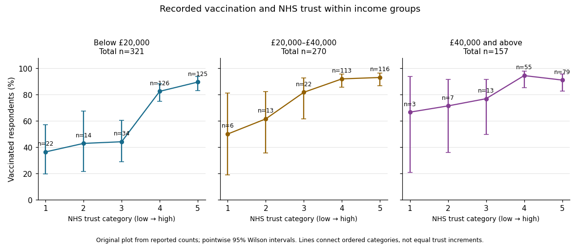

In the elaboration model, the positive direction is replicated after conditioning on income: income does not fully explain away the observed trust–vaccination relationship. The decreasing estimated contrasts and ordered coefficients suggest possible specification by income, or effect modification on an explicitly chosen scale. They do not establish it. Different p-values can arise from different sample sizes and standard errors; significant and nonsignificant results need not differ significantly. A formal statistical interaction test or a confidence interval for differences between comparable contrasts would address that question.[ref]
The Practice of Social Research (13th edition) by Earl Babbie. Chapter 15, Table 15-5: replication, specification and the causal ordering needed for explanation or interpretation
Nor do these conditional tables prove that income is a causal confounder or causal mediator. Those labels require assumptions about causal order, relevant confounding and how variables were measured. This is an observational study of recorded vaccination status, not a randomized change in trust or a test of vaccine effectiveness.
The fitted simple linear regression isIts regression slope is a predicted decrease of approximately 0.006314 trust-score units per extra year, or 0.06314 units per decade. This is an estimated statistical association between age and the score. A cross-sectional study does not establish that the same person's trust decreases at this rate as they age.
The estimated standard error of the slope is 0.005427. Testing a zero regression slope gives on 746 residual degrees of freedom and . An approximate 95% confidence interval isThere is insufficient evidence of a nonzero linear age association at the 5% level. The interval includes both small negative and small positive slopes; failure to reject does not establish an exactly zero relationship or rule out a nonlinear one.
The regression intercept 6.388920 predicts the score at age zero. That age is outside the observed 19–89 range, so interpreting it substantively would be extrapolation. Its very small reported p-value tests a zero intercept, rather than the age hypothesis. The 746 residual degrees of freedom correspond to 748 observations minus the intercept and slope.
The coefficient of determination is , so the fitted line explains approximately 0.1811% of the observed centered variation, rather than 18.11%. The adjusted coefficient of determination is approximately 0.0004732. The residual standard error is 2.602 score units, close to the reported response standard deviation; most variation remains unexplained by the fitted line. With one predictor and an intercept, the slope's F-test is the square of its Student's t-test statistic, up to printed rounding, so and agree with the slope test.
Output 6 is a residual-versus-fitted plot: its vertical coordinates should be regression residuals . The fitted values range over only approximately 5.83–6.27, as the weak slope predicts over ages 19–89. The printed scatter shows no obvious strong mean curvature or clear widening funnel, but it has marked horizontal concentrations near its extreme residual levels. An absence of obvious curvature does not prove a correct linear conditional mean, and the plot alone cannot establish homoscedasticity, independent errors or a normal distribution. A normal probability plot and residuals against observation order address different aspects. Large residuals also do not by themselves establish influential observations; regression leverage and Cook's distance matter.
There is an additional inconsistency in the original figure. The descriptive output reports observed responses between zero and ten, so residual constraints from a bounded response requireYet the printed graphic contains points around , which would imply , above the stated observed maximum. Some lower-edge points likewise imply negative responses. This is present in the original PDF, rather than introduced by the transcription. The graphic therefore cannot be treated as a fully consistent diagnostic of the reported dataset. The observations about its visible shape above describe the supplied picture; reliable model checking would require the actual fitted values and residuals.
The printed code has separate typographical problems. The displayed model call supports the intended formula with
~, and the plot needs one closing parenthesis:model1 <- lm(t_guard ~ age, data = exam)
plot(fitted(model1), residuals(model1),
xlab = "Fitted values", ylab = "Residuals")
abline(h = 0)These calls correct the syntax; they cannot be rerun on the original observations because the individual-level dataset is not supplied. The regression interpretation above uses the available numerical summaries and states the diagnostic limitation explicitly.
Articles by others on the same topic
There are currently no matching articles.