Included for its quantitative statistics and computational components. The downloaded examination release also includes associated social-science papers.[ref]
https://www.ox.ac.uk/admissions/graduate/courses/msc-social-science-of-the-internet. Official course structure and core components
Technical coverage only: this article solves question 1 of the eight-question paper dated 17 January 2020. Questions 2–8 are intentionally outside the present STEM scope. They are not unavailable-input gaps, and this article does not claim complete-paper coverage.
Oxford examination release ZIP. Exact held member:
Internet Technologies and Regulation/2019- Hilary a11572w1.pdf. Its archive filename says 2019-, but the original cover identifies Hilary Term 2020, JSSI A11572W1, Friday 17 January, 09:30–12:30.The technical discussion uses information available by 17 January 2020.
By January 2020, the Internet had retained a broadly interoperable packet-delivery substrate while acquiring substantial centralisation of services and more functionality inside communication paths. The departure is real but uneven: independent network operation, physical replication, application control and placement of security functions are different architectural dimensions. Future service design should preserve endpoint responsibility for application correctness and make any delegation of control, state or trust explicit.
Network decentralisation means that important decisions and dependencies are spread across independently controlled participants, rather than being concentrated in one indispensable operator. It is not established merely by counting machines. A distributed system can run in many locations under one administrative authority. The end-to-end principle addresses a different question: where should a function be implemented? If fully satisfying an application requirement needs knowledge available at the communicating applications, an implementation confined to the intervening network cannot replace that application-level responsibility. The two ideas often reinforce one another, because a general communication service leaves applications free to evolve, but they are not equivalent.
The original argument by Jerome H. Saltzer, David P. Reed and David D. Clark is about completeness of a system function, not a blanket prohibition on intelligent routers. Consider transferring a file whose correctness includes the bytes eventually stored at the destination. Perfect link checks do not exclude a subsequent storage error. The application still needs a check at the relevant endpoint. Local error recovery may improve efficiency, while the end-to-end check establishes the requested property over the complete path through the system. The reusable argument is that application correctness is not determined by a network trace whenever two executions can have identical network behaviour but different endpoint outcomes.[ref]
End-to-end arguments in system design by Jerome H. Saltzer and others. Author-hosted reprint, pp. 1–3: function placement and the careful-file-transfer example
This division also explains the Internet's layered network architecture. Internet Protocol provides a common packet-delivery interface across different underlying networks; it does not promise reliable, ordered application completion. Transmission Control Protocol implements a reliable ordered byte stream between its transport endpoints, but receiving bytes is still different from completing the application's intended operation. Fate-sharing places essential communication state with the hosts that depend on it, reducing the need to preserve that state in every intermediate forwarding device. A route change can then leave the endpoint state intact, provided connectivity returns and the protocol can recover before it gives up. This does not mean routers contain no state: forwarding tables are different from indispensable per-connection state.[ref]
The design philosophy of the DARPA Internet protocols by David D. Clark. §§2–4, goals, survivability and fate-sharing
The IP hourglass gives this separation an evolutionary advantage. Many applications can use the same narrow inter-network interface, while many transmission technologies can support it. An application need not redesign every intermediate network before it can introduce a new service. However, the early architecture was not an entirely flat collection of equal peers. The Domain Name System is both hierarchical and distributed, with delegated authority and replicated information. Its design replaced a centrally distributed host-name file, so some architectural developments increased distribution. A common protocol or a logically coordinated namespace is compatible with independently administered components. The relevant baseline is a set of design goals and compromises, not an earlier Internet with no servers, hierarchy or coordination.[ref]
Architectural Principles of the Internet (RFC 1958). §§2.1–2.4: common internetwork layer, end-to-end functions and distributed responsibility
[ref]Domain Names - Concepts and Facilities (RFC 1034). §§2.1–2.2 and 4.2: host-file scaling, distributed maintenance and zones
A clear departure from direct endpoint reachability is network address translation, particularly network address and port translation. A translator can let several privately addressed hosts share an externally usable address by maintaining mappings for their traffic. This helped accommodate address scarcity and could be introduced incrementally. It also made the path depend on an additional stateful intermediary: incoming traffic generally needs an appropriate mapping or explicit configuration, mappings can expire, and moving a flow to a different translator can break it unless the necessary state is available there. Two applications being willing to communicate is consequently not sufficient for connectivity. Application-specific gateways and relays may become necessary. The benefit is practical deployment; the cost is reduced address transparency and extra recovery and deployment constraints.[ref]
Traditional IP Network Address Translator (Traditional NAT) (RFC 3022). §§1–2 and 6: address/port mapping, state, route changes and limitations
Firewalls and application proxies make another important qualification to the ideal of an unrestricted path. A firewall deliberately restricts traffic according to a security policy. An application proxy can perform a function on behalf of an endpoint, sometimes with information and permissions beyond ordinary packet forwarding. Such arrangements can protect vulnerable systems or provide a useful service; treating every intervention as an architectural mistake would ignore actual security and operational requirements. The cost must nevertheless be recognised: an intermediary can become an additional failure point, a source of incompatible assumptions or an authority whose permission is needed to deploy a new application. Different endpoint operators may have conflicting objectives, so assuming universally cooperative, trustworthy hosts is insufficient as a design method.[ref]
Middleboxes: Taxonomy and Issues (RFC 3234). §1.1, §§2.9–2.15 and §4.1: forwarding versus middlebox functions, firewalls, proxies and architectural consequences
[ref]The Rise of the Middle and the Future of End-to-End (RFC 3724). §§3.1–3.3: changing trust relationships and service demands
One consequence is protocol ossification. If devices along a path recognise only familiar packet formats or alter fields in undocumented ways, changing the transport endpoints alone may not be enough to deploy a new transport protocol. An extension can fail even when the two hosts support it. This is a loss of the original freedom to innovate at the edges, rather than simply an increase in the number of network devices. By 2015 an architectural workshop had explicitly examined middlebox and interface constraints on transport evolution. A new service therefore needs a deployment strategy that accounts for real paths, including appropriate negotiation, measurement and fallback, rather than assuming every syntactically valid packet will pass.[ref]
Report from the IAB Workshop on Stack Evolution in a Middlebox Internet (RFC 7663). §§2–5 and §6.1: ossification, incentives and encapsulated transports
Application architecture has also become less decentralised in a way that is not reducible to middleboxes. A service can concentrate user accounts, authoritative data and protocol decisions in a provider while running many geographically separated servers. Cloud computing and a content delivery network can reduce the effort needed to deploy a service, improve network latency by placing content closer to users, and spread load across sites. A content delivery network can direct requests to delivery servers and use caching to keep copies near demand; the origin provider can authorise this arrangement. These are substantial engineering gains. Yet losing access to a provider's identity, configuration or authoritative data service can disable an application even while IP forwarding remains available. Geographical replication does not imply decentralised control.[ref]
A browser communicating with a central application server is not, merely for being client-server model, a violation of the end-to-end principle. The server may be exactly the application endpoint that has the necessary knowledge. The architectural concern is whether users can choose or replace that endpoint, whether independent implementations can interoperate, and what additional parties must be trusted. Internet service federation addresses the administrative dimension: independent providers communicate using an agreed protocol instead of every participant needing an account at one authority. Internet mail supplies an established example of communication across separately operated domains, even though individual organisations may use large central servers. Federation does not itself guarantee cryptographic confidentiality, fault tolerance or choice among many operators; it changes who can participate and which dependencies are mandatory.[ref]
The distinction is especially clear for encryption. Transport Layer Security protects a channel between its cryptographic endpoints; it does not define those endpoints as the two ultimate human users. In one design, a browser's TLS peer is the origin server and intermediate routers lack the channel keys. In another, the origin authorises a CDN edge to terminate TLS and the CDN edge uses a second protected channel to the origin. Both links can be encrypted while the CDN edge processes plaintext. TLS termination moves the confidentiality boundary. This is not automatically an unauthorised interception, but it is a different trust arrangement that should be documented. Network address translation alone does not require decrypting a TLS payload.[ref]
The Transport Layer Security Protocol Version 1.3 (RFC 8446). §1: channel properties between peers and dependence on application interpretation of authentication
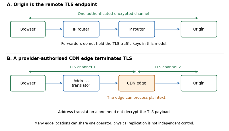
Forwarding and address translation differ from authorised TLS termination: two protected channels can expose plaintext at their shared endpoint
. Details. If a service promises secrecy from its own relay or storage provider, transport encryption to that provider is insufficient. End-to-end encryption must keep the relevant plaintext and decryption capability at the intended application endpoints. Similarly, a client can verify a publisher's digital signature on an object obtained through a cache, separating the source of delivery from the authority for content. Neither mechanism alone hides all communication metadata, solves endpoint compromise, or ensures the service is reachable. The design question is which party needs which information, and what property the user is actually promised, rather than whether every segment has an encryption label.
These changes therefore call for selective preservation of the original principles. At the network layer, favour general interfaces and independently deployable extensions rather than unnecessary application-specific assumptions. IPv6 expands the address space and can remove a reason for address sharing; it does not compel operators to permit incoming connections, remove firewalls or decentralise application ownership. It would be unjustified to expect a larger address alone to restore the whole earlier architectural ideal. Address transparency, security policy and application control require separate choices.[ref]
Internet Protocol, Version 6 (IPv6) Specification (RFC 8200). §1: expanded addressing and other changes from IPv4
[ref]Internet Transparency (RFC 2775). §§2.1–2.3, §§3.3–3.6 and §5.1: distinct end-to-end properties, intermediaries and limits of address-space remedies
At the transport layer, the November 2019 QUIC Internet-Draft provides a timely example of trying to evolve functionality at the endpoints over the widely deployed User Datagram Protocol. It includes encrypted transport machinery, connection identifiers and support for changes of network path. As of this examination it is work in progress, not a completed Internet standard. Its approach shows how deployment constraints can stimulate a new endpoint implementation, but it is not proof that every network will carry UDP or that encapsulation abolishes all middlebox dependencies. Designers must preserve congestion control and explicitly assess the tradeoff between encrypted protocol details and information needed for network operation.[ref]
At the application layer, put the final checks for the promised result at the endpoints that can actually observe it. An intermediate acknowledgement should not be confused with successful storage or completion of a user operation. When an intermediary is useful, specify its authority, its failure behaviour and the state it holds; make security-sensitive delegation visible rather than silently expanding trust. Separate this from the performance decision to use data replication or caching. Those optimisations may be valuable even when endpoint verification remains indispensable.
Resilience likewise requires examining dependencies across operators and components, not just counting replicas. Identify which failures can be tolerated while an application still makes progress, including failure of a naming, identity or configuration service. Where appropriate, use independently operated services, interoperable protocols and data portability so that users can move state or change providers. These options have costs: federation requires compatibility between implementations, while replicas need coherent handling of updates. A centrally operated component can be a reasonable choice when its benefits justify a clearly identified dependency. It should not acquire the label decentralised simply because it is replicated.
A useful evaluation would test the service from independently administered networks, including one with address translation, and distinguish connection establishment, endpoint correctness and recovery after an intermediary restart. For a delegated delivery service, separately test what an authorised CDN edge can observe and what an application-level authenticity check validates. Such tests make the architectural claims concrete; a successful throughput measurement alone cannot establish freedom from mandatory intermediaries or secrecy from a delivery provider.
The strongest January 2020 assessment is that end-to-end function placement remains a valuable criterion, while universal reachability and independent control have been constrained at several layers. The design goal for subsequent services is a clear allocation of correctness, trust and failure responsibility, with the benefits and dependencies of intermediaries exposed rather than hidden behind a simple centralised/decentralised label.
Technical coverage only: this article answers question 1 of the eight-question paper dated 11 January 2019. Questions 2–8 are outside the present STEM scope; they are not missing-input TODOs.
Source paper: Oxford examination release ZIP, member
Internet Technologies and Regulation/2018 Hilary a11572w1.pdf. The original cover identifies Hilary Term 2019 despite the archive member's 2018 label. The discussion uses information available by the examination date.The Internet still reflects the original principles strongly in its common communication substrate, while many applications concentrate decisions and essential services in fewer hands. It is therefore necessary to distinguish the location of machines, the authority to control a service, and the placement of the checks that establish its correctness. A geographically extensive service can remain centrally controlled; a service with independently operated participants still needs to establish its promised result at the relevant endpoints.
The end-to-end principle is a test of function placement. If an application's required property depends on what happens at its endpoints, placing a partial implementation in the intervening network cannot establish the whole property. A receiver can accept bytes and then fail before storing the requested file correctly. The sender therefore needs the appropriate application-layer acknowledgement, rather than treating a transport acknowledgement as proof of durable storage. In this sense, application correctness is not determined by a network trace. Local recovery can still improve performance; it complements the application check rather than replacing it.[ref]
End-to-end arguments in system design by Jerome H. Saltzer and others. Printed pp. 1–3 and 7: function placement, careful file transfer and application acknowledgements
This principle does not imply that routers must be devoid of useful functions, nor that every mechanism belongs at precisely one layer. Its benefit is a clear account of which component supplies a promised result. Internet Protocol offers a common interface across different underlying networks. The IP hourglass permits different applications above that interface and different transmission technologies below it. New application behaviour need not require every intermediate network to be redesigned.[ref]
Architectural Principles of the Internet (RFC 1958). §§2.2–2.4: internetworking, end-to-end responsibility and concentrating application intelligence at endpoints
There is nevertheless a real departure from a simple picture of directly communicating hosts. Middleboxes can inspect, alter or constrain traffic in ways that ordinary packet forwarding does not. A firewall makes a decision about permitted communication; a proxy server can become a separate application participant. Such mechanisms may address legitimate local needs, but an application's assumptions about what the path will carry now require additional justification. A new transport protocol cannot infer successful deployment merely from the existence of compatible host implementations.[ref]
Middleboxes: Taxonomy and Issues (RFC 3234). §1.2 and §2: the hourglass model and the catalogue of intermediary functions
Network address translation gives a concrete state-management example. With network address and port translation, several private hosts can share an externally visible address through mappings in an intermediary. A particular active connection can depend on the continued presence of its mapping, not just on the two host implementations. Loss of that mapping can interrupt the connection even when those hosts remain operational. This qualifies the fate-sharing goal of keeping indispensable communication state with the participants that depend on it. It does not mean every translation failure is permanent or that a service cannot establish a new connection; the interrupted operation and its recovery behaviour must be specified.[ref]
Traditional IP Network Address Translator (Traditional NAT) (RFC 3022). §§2–3: traditional NAT/NAPT mappings, session state and routing constraints
Concentration at the application layer is a separate issue. A content delivery network can place copies close to demand and direct requests to suitable delivery endpoints. This can reduce network latency and avoid repeatedly transferring the same content from its origin. Those are useful engineering results. However, geographical replication does not imply decentralised control: many delivery sites can still answer to one authority or depend on the same origin. Interconnection between delivery networks also requires explicit arrangements for request routing and metadata, rather than arising automatically from their physical distribution.[ref]
Framework for Content Distribution Network Interconnection (RFC 7336). §§1.2–3.1: actors, request redirection, content acquisition and interconnection interfaces
Users consequently need to ask which operations remain possible when a provider or shared component is unavailable. Two service replicas might hold the same data in different regions yet both require one identity provider for each new authentication. That provider is then a mandatory service dependency for the new-user operation. More replicas of the data do not remove the dependency. Already admitted users might continue to work under a different design, so the conclusion concerns the declared operation rather than every possible use of the service. This is why failure domains and service availability must be analysed through dependencies as well as geography.
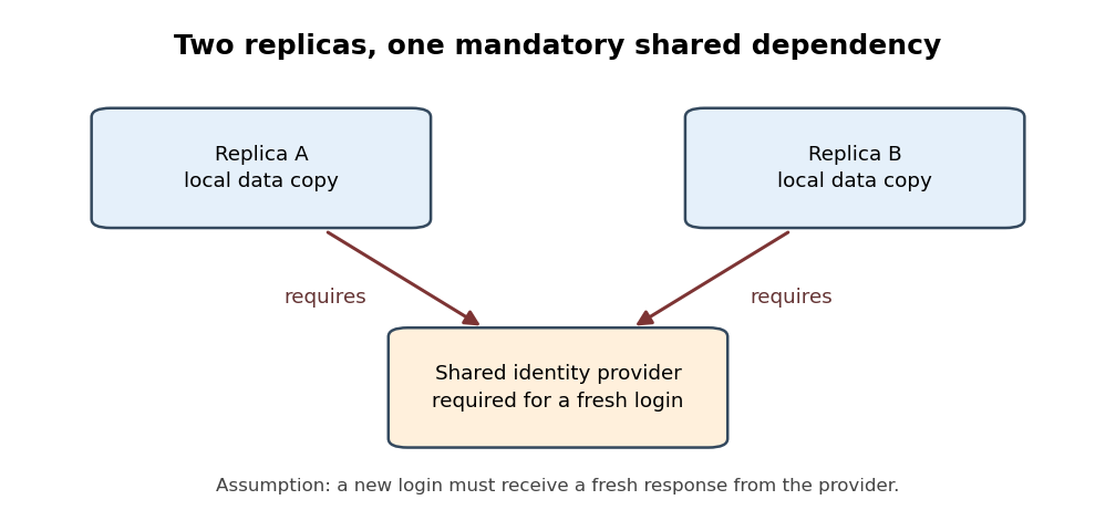
Two service replicas with one mandatory identity dependency
. Original schematic for an operation that requires a fresh identity check. An arrow points from a replica to a component whose response it requires. Loss of the shared identity provider can block that operation at both replicas even while their data remains intact; the diagram makes no claim about operations that do not require a new authentication response. Details.The endpoint boundary also determines what a security promise means. Transport Layer Security protects communication to the actual TLS peer. Version 1.3 had been standardised in August 2018, before this sitting. If an authorised CDN edge terminates that connection, it is a participant in the protected communication and can obtain the application plaintext. That can be an intentional delegation, but it cannot simultaneously promise secrecy from that same participant merely because the connection carries an encryption label. A promise of secrecy from the intermediary requires suitable end-to-end encryption with the relevant decryption capability at the intended application endpoints.[ref]
The Transport Layer Security Protocol Version 1.3 (RFC 8446). August 2018, §1 and §2: goals and the authenticated, confidential channel between TLS peers
Not every delegated function requires that stronger secrecy promise. A client might instead need to check that an object came from an identified publisher while permitting any suitable cache to deliver it. A digital signature, verified against the intended publisher's authenticated public key, can separate the delivery source from the authority for the content. It does not establish that the publisher's statements are true or make the object reachable. The useful design step is to state the promised property before deciding which component must be trusted to establish it.
For future services, one option is internet service federation: independently operated services exchange requests through compatible communication protocols.[ref]
Simple Mail Transfer Protocol (RFC 5321). §2.1 and §5: exchange between independently addressed mail systems and domain-based routing
This can permit a choice of provider, but it does not by itself eliminate shared naming dependencies or guarantee that all participants apply compatible policies. Data portability is a distinct requirement: users may need to take their state to another provider. A nominally open protocol is insufficient if the application's useful state cannot move with them.The engineering response is therefore selective. Retain endpoint checks for the promised application result, identify every mandatory service dependency, and decide explicitly where control and state should reside. Use caching, data replication and authorised intermediaries when they improve the intended service, while testing whether common dependencies defeat the expected fault tolerance. Where independent operation is a requirement, test that requirement directly rather than counting machines. This preserves the adaptable part of the original architecture without pretending that every application must have the same trust boundary or administrative arrangement.[ref]
Architectural Principles of the Internet (RFC 1958). §1 and §§2.3–3.1: architectural evolution, application responsibility and design choices
Source release: www.whatdotheyknow.com/request/admission_statistics_and_past_pa/response/2722250/attach/2/Exam%20papers.zip?cookie_passthrough=1
A null hypothesis specifies the population comparison to be tested, for example equality of the population means for women and their complement. The alternative hypothesis for a two-sided test is a nonzero difference. A Student's t-test measures an estimated difference in units of its estimated standard error:On the reported calibration, the sampling distribution under the null hypothesis is Student's t-distribution with statistical degrees of freedom. Consequently the two-sided test has p-valueWith this many statistical degrees of freedom, the Student t-distribution is close to the standard normal distribution: exceeds the approximate two-sided critical value , but falls short of the value . Using the supplied calibration, reject at the significance level, but not at . The large statistical degrees of freedom justify this comparison; a value need not be significant for an arbitrary very small number of statistical degrees of freedom.
The p-value is the probability, under the specified null hypothesis and sampling assumptions, of a test statistic at least as discrepant as the observed one. It is not the probability that the null hypothesis is true, nor the probability that the observed difference happened “by chance”. A significance level of controls the long-run type I error rate of the testing procedure when its assumptions hold. Failing to reject at does not prove equality. Statistical significance also does not measure the substantive size or importance of a difference.
The reported sample means place the women's mean scale units above the overall mean. The negative test statistic can reflect the order of subtraction; it does not reverse that observed ordering. An appropriate pre-specified directional one-sided test would have a tail p-value approximately on the supplied calibration, but one cannot choose that direction after inspecting the results simply to halve a p-value.
There is a design issue behind the numerical calculation: the women are included in the overall sample. Comparing a subgroup mean with its containing sample mean requires accounting for shared observations. If is the women's sample fraction and the mean for the remaining respondents, thenThese two estimates are not independent. An ordinary independent-two-sample Student's t-test of women against the entire respondent sample would therefore use an inappropriate standard error. The interpretation above accepts the supplied test statistic and its stated null calibration; a valid analysis of the underlying data should compare disjoint groups, or calculate the shared-sample covariance correctly. The summary alone cannot establish which calculation was used. Simple random sampling supports sampling inference under the stated design, but an observed gender association does not establish a causal effect.
Each row of the contingency table is a conditional distribution of the safety category among respondents with that experience status. Thus the relevant comparison uses row percentages, rather than interpreting the larger number of respondents with some bad experiences as itself an effect on safety.
The sample proportions reporting feeling very safe are without bad experiences and with some bad experiences: the latter is lower by about percentage points. Feeling fairly safe rises from to , a difference of about percentage points. Feeling unsafe changes only from to , about percentage points. The main descriptive shift is therefore from very safe toward fairly safe, rather than a large increase in the unsafe category.
Pearson's chi-squared test tests the null hypothesis that experience status and safety category are independent. If that were true, the expected cell count would be its row total times column total divided by . The Pearson chi-squared statistic sums squared observed-minus-expected count differences divided by their expected counts. HereThe expected counts are comfortably large, with minimum approximately , so the ordinary large-sample chi-squared distribution approximation is appropriate under the sampling assumptions. There is evidence against independence even at the significance level. The reported likelihood-ratio result gives the same conclusion.
Magnitude is a separate question. Cramér's V giveswhich describes a weak statistical association. It does not mean that of safety is explained. Nor does the p-value measure the size of that association.
For ordinal direction, order the experience categories as none, some, and the safety categories from very safe toward unsafe. Goodman and Kruskal's gamma compares concordant pairs with discordant pairs after excluding tied pairs:Its small positive sign then corresponds to a weak tendency toward less safety among respondents with bad experiences. The sign would reverse if exactly one category ordering were reversed. Because this contingency table has many ties, the response-direction Somers' D, which retains response ties among pairs with different predictor values, is smaller:These coefficients describe ordered association; the omnibus Pearson's chi-squared test tests any departure from independence and does not supply a separate p-value for gamma.
The column-dependent Goodman and Kruskal's lambda makes the weak predictive improvement tangible. Predicting the overall most frequent safety category makes errors in this table. Using a separate most frequent category within each experience row makes , giving , only about a reduction in those classification errors.
The sample supports a statistically detectable but weak association, chiefly a reduced sample proportion feeling very safe. This observational study does not establish that bad experiences cause the change: reverse direction, reporting differences or confounding could also contribute. The numerical p-value also presumes the sampling and complete-case assumptions appropriate to the observations used.
Conditioning on marital status produces five contingency tables. In each, compare the conditional row percentages. The following differences are the sample proportion with some bad experiences minus the sample proportion without them, in percentage points; negative very-safe differences mean fewer respondents feeling very safe in the former group.
| Marital-status stratum | Difference: very safe | Difference: unsafe | Reported Pearson's chi-squared test p-value | Cramér's V | Goodman and Kruskal's gamma |
|---|---|---|---|---|---|
| Single | |||||
| Married | |||||
| Living with a partner | (inconsistent; see below) | ||||
| Divorced | |||||
| Widowed |
The p-values test independence within the respective strata; the magnitudes and directions come from the conditional percentages and association measures. Differences in the table are calculated from the counts before rounding.
Among single respondents, the very-safe sample proportion changes from to , while the unsafe sample proportion changes from to . The direction resembles the weak pooled pattern, but supplies little evidence against independence in this stratum. This is not evidence that the population association is exactly zero.
Among married respondents, the very-safe sample proportion changes from to and the fairly-safe sample proportion rises from to . Unsafe remains almost unchanged, versus . Thus the within-stratum association again chiefly shifts very safe toward fairly safe. Its is below the significance level, while still indicates a small association.
For respondents living with a partner, very safe changes from to , fairly safe from to , and unsafe from to . The very-safe difference is larger than in the married stratum. The printed p-value would be just below the conventional significance level. However, this particular output is internally inconsistent: recalculating Pearson's chi-squared test from its six displayed counts gives , , and . The reported agrees with the counts, whereas the printed would itself imply for two statistical degrees of freedom, rather than the printed . Using the displayed counts, this stratum does not reject independence at . The source PDF itself contains these incompatible figures; this is not resolved by rounding.
Among divorced respondents, very safe changes from to , but unsafe also decreases, from to , as fairly safe increases from to . This is a redistribution toward the middle category, not a simple shift toward greater unsafety. The near-zero gamma, , reflects the lack of a consistent ordinal direction, while can still register distributional differences without a direction. The p-value does not reject independence.
Among widowed respondents, very safe changes from to , and unsafe from to . The ordinal association is positive on the chosen ordering, with gamma . Its lack of conventional statistical significance, , does not imply a smaller estimated association than in the married group: the widowed stratum has only complete observations, versus in the married stratum, and therefore less precision. All five tables have sufficiently large expected counts for the reported approximations; even the smallest expected count is about .
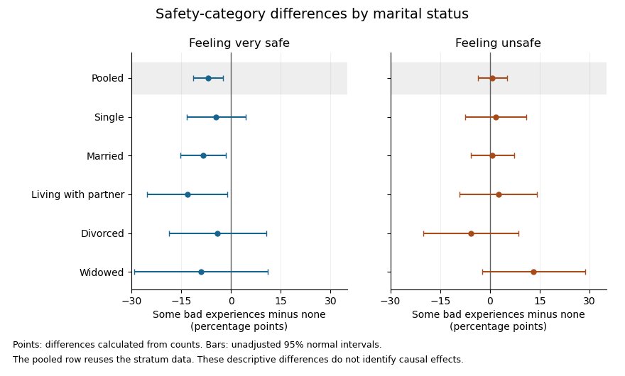


The plot uses large-sample Wald confidence intervals for the difference of independent sample proportions within each stratum. They concern the individual category contrasts, whereas the tabulated Pearson's chi-squared tests compare the full three-category distributions. The intervals are unadjusted for multiple hypothesis testing; the pooled row reuses the stratum observations, so it is not a sixth independent sample.
In the elaboration model, the persistence of a generally weak positive ordinal pattern within four strata is closer to partial replication than to a complete explanation of the pooled association by marital status. The differences in estimated patterns suggest possible specification: the divorced group's shift toward the middle category differs from the widowed group's shift toward unsafe. They do not by themselves establish population effect modification. In particular, significant and nonsignificant results need not differ significantly; compare the effects using an interaction contrast or a fitted model with the appropriate interaction terms, rather than comparing their separate p-values.[ref]
The Difference Between Significant and Not Significant is not Itself Statistically Significant by Andrew Gelman and Hal Stern. Printed p. 328, Introduction: comparing significance labels does not test the difference between estimates
One additional omnibus check can be derived from the supplied tables without assuming a common effect. Recalculating the five statistics from the counts, including the corrected living-with-partner statistic, the joint conditional independence test for stratified contingency tables givesUnder independent-stratum sampling this tests independence within every stratum jointly; it does not test whether the association is homogeneous across strata. It does not reject at , but this alone does not establish that stratification removed the population association: its ten-degree-of-freedom alternative is less focused than the pooled two-degree-of-freedom test, and nonrejection is not proof of equality.
The elaboration model also distinguishes an antecedent confounder from an intervening causal mediator. These cross-sectional tables do not establish the relevant time ordering or identify either role for marital status. Five separate stratum tests further require caution about multiple hypothesis testing: for example a Bonferroni correction at familywise would use per test, below all five individual p-values. That caution changes the interpretation of selected significance labels, not the observed conditional percentages.
The estimated patterns vary across strata, but the tables neither establish a population interaction nor prove that marital status explains away the association.
The ordinary least squares fit estimates the conditional mean of the continuous safety response as a linear function of the income coding:The regression coefficient for income is positive. Since larger response values mean greater safety, one additional coded income unit corresponds to an estimated increase of safety-scale units in the fitted mean. Following the question's stated units, a unit is a £10,000 income step. The observed coding also uses income bands with open end categories, so this is a linear trend per coded band step; it is not evidence of a known constant effect for every extra pound, especially within the open top band. The output's abbreviated variable label does not override the stated units.
The intercept is the fitted mean at income code zero. It is estimated as , but zero is outside the observed income codes, so that value is an extrapolated model baseline, not an observed estimate for a particular income category. Its small p-value tests a zero intercept; it is not the main test of the income association.
For the income coefficient, the standard error is . The reported test statistic and two-sided test giveproviding strong evidence against the null hypothesis of zero linear slope under the stated model assumptions. A Student t confidence interval, using residual statistical degrees of freedom, isThis is an interval for the population linear coefficient under the model, not an interval containing of individual safety scores. The large-sample estimate is precise enough to detect a positive association, but that does not establish substantial individual predictive power.
The coefficient of determination is : the fitted line accounts for about of the in-sample variation about the response sample mean. The adjusted coefficient of determination is about . Thus income alone explains very little of the observed variation, despite the small slope p-value. The residual standard error of response units describes substantial scatter about the fitted line. This is an estimated residual standard deviation, rather than the standard error of the slope or a complete individual prediction interval.
The overall F-test has on statistical degrees of freedom and . With one predictor and an intercept, it tests the same zero-slope hypothesis as the coefficient Student's t-test; , up to rounding. It is not an additional independent confirmation. In this simple linear regression, the Pearson correlation coefficient has the slope's sign and magnitude , another description of the weak linear association.
The regression uses complete observations and estimates two coefficients, giving residual statistical degrees of freedom. The deletion of observations is complete-case analysis; extending its conclusions to the full target population requires suitable assumptions about the missing-data mechanism. Classical reported standard errors also rely on an adequate linear conditional mean, independent errors and homoscedasticity; a normal linear model gives the finite-sample Student t-distribution and F-test calibration, while large-sample approximations can justify similar tests under weaker distributional assumptions. The printed summary alone does not establish these assumptions. Regression diagnostics and, where appropriate, heteroskedasticity-consistent standard errors address different parts of that assessment.
Finally, this unadjusted observational study estimates an association. Other covariates, such as age or experience status, may be related to both income and reported safety. Without additional design or causal identification assumptions, the positive fitted slope does not establish that increasing income would cause an increase in safety.
Source paper: released examination archive. The cover identifies Michaelmas Term 2022. All four questions are addressed; statements and the original residual figure are omitted. The supplied tables concern trust and recorded vaccination status; they do not support the introduction's separate reference to gender or vaccine willingness. The inconsistent residual graphic and a qualification about the first test's degrees of freedom are discussed where they matter.
Let and be the population means of the newspaper trust score for the unvaccinated and vaccinated groups. A two-sided hypothesis test comparesThe observed difference of sample means is : the vaccinated group has a one-unit higher average trust score. The negative test statistic agrees with subtraction in this order. A Student's t-test scales the estimated difference by its estimated standard error; means that the observed difference is 3.6 estimated standard errors below the equal-mean null hypothesis.
Using the reported reference Student t-distribution with 747 statistical degrees of freedom,Thus the equal-mean null hypothesis is rejected at a prespecified 5%, 1% or 0.1% significance level, subject to the test's assumptions. A p-value is a probability of a result at least this extreme under the specified null hypothesis and sampling model. It is neither the probability that the null hypothesis is true nor the probability that this particular conclusion is mistaken. A chosen significance level controls the procedure's type I error probability under that model.
The estimated difference is more informative than statistical significance alone. If the reported statistic uses this one-unit contrast, its estimated standard error is . The corresponding approximate 95% confidence interval isThis interval concerns a population mean difference under repeated sampling; it is not a range containing 95% of individual trust scores. Its practical interpretation also depends on the trust scale and the importance of a one-unit difference.
The groups are disjoint, so an independent-samples comparison is appropriate if the sampled observations are independent. The exact pooled Student's t-test additionally assumes common population variance and normal distributions; Welch's t-test permits unequal variances and uses an approximate reference distribution. A bounded or ordinal rating need not be exactly normal, so treating it numerically and using a large-sample approximation also requires judgment about group sizes and the score's meaning.
There is a bookkeeping qualification. The later outputs use 748 observations. If these are also the complete observations for this two-group comparison, the pooled test has statistical degrees of freedom, and the Welch degrees of freedom upper bound is also 746. The printed 747 therefore needs the original test call or a different sample count to reconcile it. The reported-calibration calculation above answers the stated test; it does not invent group sizes or silently change the reference distribution.
The evidence supports an association between higher newspaper trust and recorded vaccination, rather than a causal effect of trust. An observational study does not rule out confounding, selection bias or reverse causation. A statistical hypothesis test cannot supply those missing causal assumptions.
These are row percentages, so the comparisons estimate the conditional probability of recorded vaccination within each NHS trust category. The percentages increase across the ordered trust categories asThe extreme-category difference is approximately 49.31 percentage points, rather than a 49.31% relative increase. The ordinal categorical variable records an order; the categories do not establish equal numerical trust increments.
Under the null hypothesis of independence, the expected count in a cell is its row total times its column total divided by 748. The Pearson chi-squared statistic compares observed and expected counts throughThere are statistical degrees of freedom, giving . The minimum expected count is approximately 5.015, so the usual expected-count concern is much less acute here than in the income strata. The table gives strong evidence of a statistical association. The likelihood-ratio test of independence in a contingency table agrees: its statistic is approximately 81.361 on four statistical degrees of freedom, with a very small p-value. The displayed
0.000 is rounding, not a zero probability.For magnitude, Cramér's V isIt describes the size of the departure from independence without using the category order or giving a direction. Calling it “moderate” is only a rough contextual description; the actual percentage differences are easier to interpret.
The ordered coefficients describe a positive direction. Goodman and Kruskal's gamma uses only concordant pairs and discordant pairs:It excludes tied pairs, which are frequent when the response has only two categories. It is therefore not a claim that 54.7% of respondents were vaccinated because of their trust. The directional Somers' D for vaccination as response includes pairs tied on that response in its denominator:The smaller value reflects the retained ties; it does not contradict the positive statistical association.
The small column-dependent Goodman and Kruskal's lambda has a useful prediction interpretation. Without trust information, always predicting the more frequent vaccinated category gives 121 mistakes. Predicting the majority category separately in each trust row gives mistakes. HenceTrust reduces this particular modal-prediction error by only about 4.13%, despite the strong evidence against independence. Most rows retain the same majority category. Evidence of association, its ordinal direction and improvement in a chosen prediction rule are different questions. None establishes that changing trust would change an individual's vaccination status.
The association remains positive within each income group, although its estimated size is smaller in the higher-income groups. The two extreme trust categories give the following conditional vaccination percentages and differences:
| Annual household income | Lowest trust | Highest trust | Difference in percentage points |
|---|---|---|---|
| Below £20,000 | 36.36% | 89.60% | 53.24 |
| £20,000–£40,000 | 50.00% | 93.10% | 43.10 |
| £40,000 and above | 66.67% | 91.14% | 24.47 |
In the lowest-income group, the intervening percentages are 42.86%, 44.12% and 82.54%, so the increase is monotone. Its Pearson chi-squared statistic is approximately 62.520 on four statistical degrees of freedom, with the printed asymptotic . Cramér's V is approximately 0.441, Goodman and Kruskal's gamma is approximately 0.626 and the column-dependent Somers' D is approximately 0.259. The column-dependent Goodman and Kruskal's lambda is approximately 0.158: trust improves the modal prediction more here than in the pooled table.
In the middle-income group, the intervening vaccination percentages are 61.54%, 81.82% and 92.04%. The printed Pearson chi-squared statistic is approximately 24.033 on four statistical degrees of freedom, with asymptotic . Cramér's V is approximately 0.298, Goodman and Kruskal's gamma approximately 0.454 and column-dependent Somers' D approximately 0.100. Column-dependent Goodman and Kruskal's lambda is zero: vaccinated respondents are the majority in every row, so the modal prediction never changes. A zero lambda does not mean independence.
In the highest-income group, the intermediate vaccination percentages are 71.43%, 76.92% and 94.55%; the final category falls slightly to 91.14%. Thus the observed pattern is broadly positive rather than strictly monotone. The printed Pearson chi-squared statistic is approximately 8.199 on four statistical degrees of freedom, with asymptotic . It does not reject independence at 5%. The corresponding Cramér's V is approximately 0.229, Goodman and Kruskal's gamma approximately 0.281 and column-dependent Somers' D approximately 0.058. The column-dependent Goodman and Kruskal's lambda is again zero.
Small counts limit the asymptotic tests, especially in the middle- and highest-income tables. Their minimum expected counts are approximately 0.644 and 0.306, with respectively 30% and 40% of cells below five. The lowest-income table has one expected count below five, with minimum approximately 3.315. These diagnostics concern expected counts under independence, not just the observed row sizes.
The supplied counts are sufficient to make an exact conditional Pearson test for a binary contingency table, without needing individual records or assuming a chi-squared distribution approximation. Conditioning on the row totals and total unvaccinated count removes the common unknown binomial probability. For each admissible table, sum its multivariate hypergeometric distribution probability when its Pearson chi-squared statistic is at least the observed one. Complete enumeration gives:
| Income group | Enumerated tables | Exact conditional p-value |
|---|---|---|
| Lowest | 507150 | |
| Middle | 22379 | |
| Highest | 2585 |
These are new exact conditional calculations, rather than the paper's printed asymptotic p-values. They confirm evidence of association in the first two groups and nonrejection at 5% in the third, while showing the numerical effect of sparse cells. The tail is ordered by the Pearson chi-squared statistic; an exact test with a different ordering need not have the same p-value. Fixed-margin Monte Carlo tests approximate this same Pearson-ordered tail when enumeration is impractical.[ref]
Pearson's Chi-squared Test for Count Data in the R documentation. Details: fixed-marginal simulation for contingency-table Pearson tests
The original count-based figure below includes pointwise approximate 95% Wilson intervals. The very wide intervals for sparsely populated trust categories make the uncertainty visible; they are not simultaneous intervals or a formal test of differences between income groups.
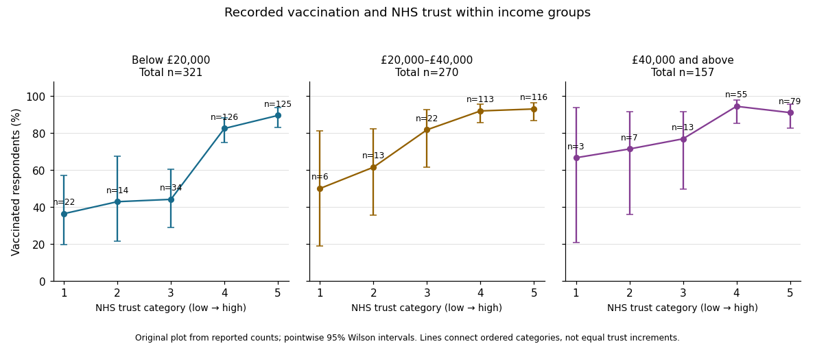

In the elaboration model, the positive direction is replicated after conditioning on income: income does not fully explain away the observed trust–vaccination relationship. The decreasing estimated contrasts and ordered coefficients suggest possible specification by income, or effect modification on an explicitly chosen scale. They do not establish it. Different p-values can arise from different sample sizes and standard errors; significant and nonsignificant results need not differ significantly. A formal statistical interaction test or a confidence interval for differences between comparable contrasts would address that question.[ref]
The Practice of Social Research (13th edition) by Earl Babbie. Chapter 15, Table 15-5: replication, specification and the causal ordering needed for explanation or interpretation
Nor do these conditional tables prove that income is a causal confounder or causal mediator. Those labels require assumptions about causal order, relevant confounding and how variables were measured. This is an observational study of recorded vaccination status, not a randomized change in trust or a test of vaccine effectiveness.
The fitted simple linear regression isIts regression slope is a predicted decrease of approximately 0.006314 trust-score units per extra year, or 0.06314 units per decade. This is an estimated statistical association between age and the score. A cross-sectional study does not establish that the same person's trust decreases at this rate as they age.
The estimated standard error of the slope is 0.005427. Testing a zero regression slope gives on 746 residual degrees of freedom and . An approximate 95% confidence interval isThere is insufficient evidence of a nonzero linear age association at the 5% level. The interval includes both small negative and small positive slopes; failure to reject does not establish an exactly zero relationship or rule out a nonlinear one.
The regression intercept 6.388920 predicts the score at age zero. That age is outside the observed 19–89 range, so interpreting it substantively would be extrapolation. Its very small reported p-value tests a zero intercept, rather than the age hypothesis. The 746 residual degrees of freedom correspond to 748 observations minus the intercept and slope.
The coefficient of determination is , so the fitted line explains approximately 0.1811% of the observed centered variation, rather than 18.11%. The adjusted coefficient of determination is approximately 0.0004732. The residual standard error is 2.602 score units, close to the reported response standard deviation; most variation remains unexplained by the fitted line. With one predictor and an intercept, the slope's F-test is the square of its Student's t-test statistic, up to printed rounding, so and agree with the slope test.
Output 6 is a residual-versus-fitted plot: its vertical coordinates should be regression residuals . The fitted values range over only approximately 5.83–6.27, as the weak slope predicts over ages 19–89. The printed scatter shows no obvious strong mean curvature or clear widening funnel, but it has marked horizontal concentrations near its extreme residual levels. An absence of obvious curvature does not prove a correct linear conditional mean, and the plot alone cannot establish homoscedasticity, independent errors or a normal distribution. A normal probability plot and residuals against observation order address different aspects. Large residuals also do not by themselves establish influential observations; regression leverage and Cook's distance matter.
There is an additional inconsistency in the original figure. The descriptive output reports observed responses between zero and ten, so residual constraints from a bounded response requireYet the printed graphic contains points around , which would imply , above the stated observed maximum. Some lower-edge points likewise imply negative responses. This is present in the original PDF, rather than introduced by the transcription. The graphic therefore cannot be treated as a fully consistent diagnostic of the reported dataset. The observations about its visible shape above describe the supplied picture; reliable model checking would require the actual fitted values and residuals.
The printed code has separate typographical problems. The displayed model call supports the intended formula with
~, and the plot needs one closing parenthesis:model1 <- lm(t_guard ~ age, data = exam)
plot(fitted(model1), residuals(model1),
xlab = "Fitted values", ylab = "Residuals")
abline(h = 0)These calls correct the syntax; they cannot be rerun on the original observations because the individual-level dataset is not supplied. The regression interpretation above uses the available numerical summaries and states the diagnostic limitation explicitly.
Source paper: released examination archive, member Digital Social Research Statistics Core/2021 Michaelmas a14564w1.pdf. The cover identifies 9 December 2021; the reported survey was collected in October 2020. The five-category agreement item and numerical willingness scale are treated as separate reported measurements.
Let be the population means of the numerical vaccination intention score in the two recorded groups. The two-sided hypothesis test comparesThe sample means are and , giving a difference of sample means of approximately 0.01988 score points, in the order group zero minus group one. The reported group counts are 1,866 and 262; seven observations have a missing group indicator.
Welch's t-test divides that estimated difference by its estimated standard error. Its reported test statistic is , with approximately statistical degrees of freedom. This is an unequal-variance comparison; fractional statistical degrees of freedom are appropriate for the Welch approximation. The two groups need not have equal sample sizes or equal population variances.[ref]
Two-Sample t-Test for Equal Means by National Institute of Standards and Technology. Section 1.3.5.3, unpaired test statistic, unequal-variance standard error, and Welch–Satterthwaite degrees of freedom
The reported p-value is . Under the specified equal-mean null hypothesis and sampling model, a p-value measures the probability of a result at least as extreme as the observed one. It is not a posterior probability that the null hypothesis is true. There is no rejection at a prespecified 5% significance level. The observed difference of sample means is tiny relative to its estimated standard error.
The 95% confidence interval is approximatelyIt includes zero and differences in either direction. The interval's coverage refers to repeated use of the procedure under its assumptions, rather than to a probability assigned to this fixed unknown parameter or to the spread of individual scores. Nonrejection does not establish that the two population means are identical.
Simple random sampling supports the sampling interpretation, but the score is bounded and its raw distribution need not be a normal distribution. The large group sizes can support an approximate normal sampling distribution of the sample means under regularity conditions. The supplied observational study does not identify a causal explanation of any difference, and the numeric coding of the group labels creates no biological or ordinal interpretation.
Under the question's stipulated nonzero population difference, failing to reject is a type II error. A type I error would instead reject a true equal-mean null hypothesis. The premise concerns the underlying difference: another study's statistical significance, by itself, would not prove that its conclusion is correct.
For a specified alternative and sampling design, writeThe second probability is statistical power. Across repeated random samples under that same alternative and design, the long-run frequency of this kind of error is .
No numerical value of follows from this output. It depends on the true effect size, group variances, sample sizes, decision rule and chosen significance level. In particular, it is neither , nor , nor automatically 5%. The reusable result that a p-value does not determine the type II error probability demonstrates this directly in a simple normal testing model.
A small effect size or an imprecise estimator can produce low statistical power. The present confidence interval describes the precision of the estimated difference; it does not supply the missing true alternative needed to calculate the power function. A specified 5% significance level concerns the type I error rate under the null, rather than a universal error rate whenever a result is nonsignificant.
Each frequency table describes a marginal distribution, rather than a relationship among variables. The recorded two-category gender variable has 1,042 male and 1,093 female responses: 48.81% and 51.19%. It is a nominal categorical variable. Its ordering in the table supplies no quantitative ranking; a cumulative percentage over those arbitrarily ordered labels has no invariant substantive meaning.
Household income is an ordinal categorical variable with six bands. Their shares, from the lowest band upward, are , , , , and . The highest band alone contains 1,105 respondents, slightly more than half the sample. The bands are not a numerical income measurement with equal steps: the top band is open-ended, so an exact sample mean income cannot be recovered from these category counts alone.
The agreement item is also an ordinal categorical variable. Combining the first two categories givesNeutral responses account for ; the two disagreement categories together account for . These percentages describe the measured vaccination intention item, rather than actual vaccination status.
All three tables have 2,135 valid observations and no missing values for these variables, so their percentages and valid percentages coincide. This is different from the seven missing group-indicator values in question 1. The income and agreement columns sum to because the displayed percentages were rounded separately. That rounding is compatible with counts summing exactly to 2,135.
The tables alone cannot show whether the gender composition differs by income, or whether vaccination intention differs between groups. Those are questions about a joint contingency table and its conditional probabilities, not about separate marginal distributions.
The displayed percentages use row denominators. The relevant comparison is therefore the conditional probability of each response within each recorded gender group, rather than the gender composition within a response category.
For the male group, strongly agree and agree. For the female group, the corresponding percentages are and . Combining the two agreement categories givesThe female group has more neutral responses, versus , and a higher combined disagreement percentage, versus . Thus the observed distributions differ in more than a single cell.
The Pearson chi-squared test assesses the null hypothesis of independence in the complete contingency table. Under that null, the expected frequency in a cell is its row total times its column total divided by 2,135. Recalculation givesThe reported p-value, approximately , gives very strong evidence against independence under the test's sampling assumptions. The minimum expected frequency is about , so sparse expected cells are not a problem here. The test concerns the full five-category distribution, not just the combined agreement comparison.
Cramér's V summarizes the magnitude without imposing an ordering on the gender labels:The small p-value does not imply a nearly deterministic relationship. For example, the column-dependent Goodman and Kruskal's lambda is only about : choosing the modal response separately within the two groups reduces prediction errors from 1,546 to 1,506, a relative reduction of .
The positive Goodman and Kruskal's gamma must be interpreted using the table's chosen ordering. The agreement categories run toward less willingness, and gender has no intrinsic ordinal direction. A sign attached to an arbitrary group coding cannot replace the substantive comparison of conditional probabilities.
The NaN displayed for the likelihood-ratio calculation is not a valid p-value and is not evidence of no association. The Pearson chi-squared statistic can be independently recomputed from the positive cell counts. None of these calculations identifies a causal effect; the table has not controlled for income or other possible confounders.
For each income band, compare the response distribution within the two gender groups. The table below combines agree and strongly agree only to make one comparable contrast visible. The Pearson chi-squared statistic and its p-value still use all five original response categories, with four statistical degrees of freedom in every band. Income labels are thousands of USD per year; finite upper bounds are excluded.
| Income band | Male agreement | Female agreement | Difference in percentage points | Cramér's V | |||
|---|---|---|---|---|---|---|---|
| Under 10k | 117 | 38.64% | 34.25% | 4.39 | 3.433 | 0.4881 | 0.171 |
| 10k–20k | 212 | 35.90% | 35.07% | 0.82 | 5.457 | 0.2435 | 0.160 |
| 20k–30k | 245 | 52.17% | 39.22% | 12.96 | 5.893 | 0.2073 | 0.155 |
| 30k–40k | 278 | 54.90% | 37.50% | 17.40 | 10.117 | 0.03851 | 0.191 |
| 40k–50k | 178 | 54.74% | 38.55% | 16.18 | 6.687 | 0.1534 | 0.194 |
| 50k and above | 1105 | 71.16% | 50.21% | 20.95 | 63.765 | 0.240 |
In the lowest-income band, combined agreement differs by only about percentage points. The full distributions still differ descriptively: strong disagreement is in the male group and in the female group. The omnibus Pearson chi-squared test does not reject independence at 5%, but that decision does not prove equal distributions.
In the 10k–20k band, combined agreement is almost the same. Nevertheless, strong agreement is higher in the female group, versus , while the less intense agreement category is higher in the male group, versus . Collapsing the categories hides that distinction. The full-distribution p-value is approximately .
In the 20k–30k band, combined agreement is higher in the male group by about percentage points. Strong agreement alone is versus . The observed difference is therefore larger than in the two lowest bands, despite its full-table p-value remaining above 5%.
In the 30k–40k band, combined agreement differs by about percentage points, with fewer male neutral responses, versus . The full-table p-value of is nominally significant at 5%. In the 40k–50k band, the combined agreement gap is a similar percentage points, but the full-table p-value is . These labels are not a direct comparison between the two effects: significant and nonsignificant results need not differ significantly.
In the highest-income band, strong agreement is in the male group and in the female group. Combined agreement differs by about percentage points. This band has both the largest sample size and the largest Cramér's V of the six tables, with a very small p-value. Its particularly strong evidence reflects both precision and an observed difference in the distribution.
All six minimum expected frequencies exceed five: approximately , , , , and . Thus sparse expected counts do not provide a reason to reject the usual chi-squared distribution approximation here. If the six hypothesis tests form one exploratory family, a Bonferroni correction would use for each test; only the highest-income result crosses that threshold. This qualifies the unadjusted 30k–40k result without turning its observed contrast into zero.
In the elaboration model, the larger agreement gaps in the middle and upper bands provide a descriptive pattern of specification: the conditional contrast varies with income. This is not a Simpson's paradox reversal, because the combined agreement difference has the same sign in every band. Nor is the larger high-income effect size established simply by comparing its p-value with the other p-values. A formal claim of effect modification requires a stated scale and an appropriate comparison of the effects.
The pooled comparison also mixes different income compositions. The highest-income band contains of the male group but of the female group. Average each group's six agreement proportions over the same pooled income weights using standardization with common weights. This givesThe crude difference was percentage points, so common weighting attenuates it by about percentage points but leaves a substantial descriptive contrast. With average-group rather than pooled-person weights, the symmetric decomposition of a stratified mean difference instead gives an exact split into approximately percentage points from conditional contrasts and percentage points from composition. These are different explicitly defined descriptive summaries, not estimates of a causally mediated share.
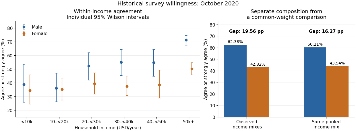

An antecedent income variable could be considered in a confounding explanation, whereas an income variable on an assumed causal pathway would enter an interpretation through causal mediation. The conditional tables do not distinguish these causal structures. They also do not identify whether any adjustment introduces collider bias. The supported conclusion is income-dependent descriptive association plus a measurable composition difference, with causal interpretation left conditional on additional assumptions.
The fitted simple linear regression for the numerical vaccination intention scale isHere age is measured in years. The fitted mean increases by about 0.01649 score points per year, or 0.16489 points per decade. The regression coefficient is an association across respondents, not an estimate of how an individual would change on ageing or of a causal effect of age.
The standard error of the age regression coefficient is . Dividing gives , with 2,133 residual statistical degrees of freedom, corresponding to fitted residual degrees. The reported two-sided p-value is , so the zero-slope null hypothesis is rejected at a prespecified 5% level, but not at 1%. An approximate 95% confidence interval isIts positive endpoints are consistent with the test decision; they do not make the slope large.
The coefficient of determination is , so the fitted age trend accounts for only 0.2744% of the observed score variation, compared with an intercept-only prediction. Its adjusted value is . In an intercept-containing simple linear regression, the positive slope implies a positive Pearson correlation coefficient . The reported overall statistic, on one and 2,133 degrees of freedom, agrees with the squared slope test statistic up to printed rounding.
The residual standard deviation estimate is score points, much larger than the fitted decade contrast. At age 50 the fitted value is about , and at 60 it is about . Across the observed ages 19 to 91, the fitted mean changes by only points. Statistical detection with 2,135 observations therefore coexists with weak individual prediction.
The intercept predicts at age zero, outside the observed age range; it should not be given a substantive infant interpretation. Centring age at its observed sample mean, , giveswhich agrees with the reported score sample mean of after rounding. The bounded scale and upper quartile at its maximum motivate attention to a possible ceiling effect; they do not establish homoskedasticity, a normal error distribution or a satisfactory linear conditional mean. Five residual quantiles cannot replace a residual plot or checks of the sampling assumptions.
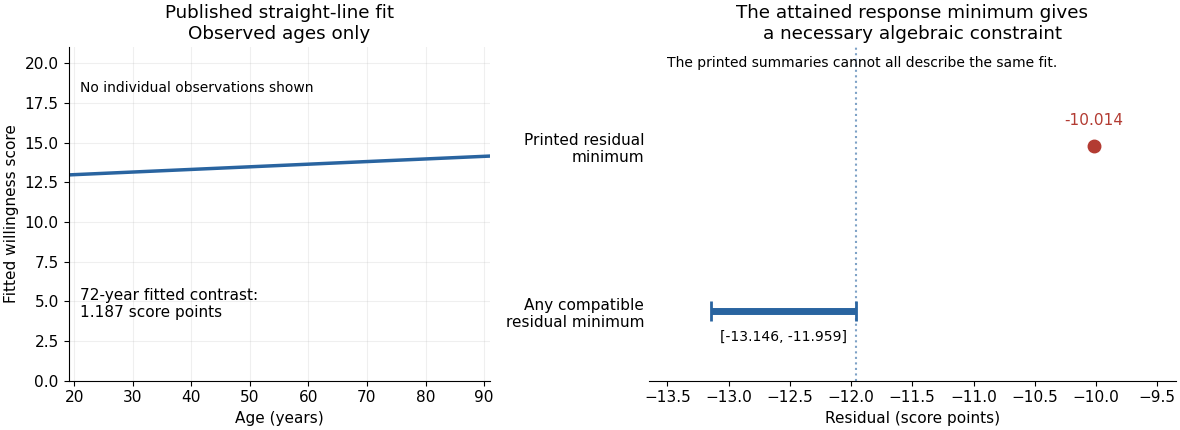
There is also a source consistency problem. The output reports that all 2,135 records have age and score present, that the attained minimum score is one, and that ages lie between 19 and 91. The positive fitted slope therefore places every fitted value between and . By residual extrema when response extrema are attained, the minimum regression residual must satisfyAt the observation with score one, its residual is already at most . The printed minimum residual, , lies outside this necessary interval. Those summaries cannot all describe the same complete sample and fitted model. The discrepancy is too large to be explained by the displayed rounding. It is present in the original PDF; the individual records would be needed to establish which printed item is wrong.

Oxford examination release ZIP. The held member is
Digital Social Research Statistics Core/2020 Trinity a14564w1.pdf; the sitting is 5 June 2020, A14564W1.The original output contains internal contradictions. Each solution distinguishes a conditional reading of a printed field from calculations based on the actually displayed counts. All six questions are covered; no unprinted age category or individual dataset is reconstructed.
Taken at face value, the printed two-sided p-value rejects equality of average political efficacy at the 5% level, with the non-employed group scoring higher. The effect magnitude and strength of evidence cannot be reported as one coherent result because the estimates, interval, test statistic and p-value contradict one another.
Let and be the expected political efficacy scores in the two employment groups in the target population. The null hypothesis is and the two-sided alternative hypothesis is . A Welch's t-test compares the difference of sample means with its standard error, estimating the two group variances separately:The reference Student t-distribution has approximate, generally noninteger statistical degrees of freedom; it does not require equality of the two variances. Observations should be independent, with finite group variances; normal distributions give the usual small-sample rationale, while large samples permit an approximate normal sampling distribution under suitable conditions. A large sample cannot correct a biased sampling procedure or dependence between observations.[ref]
Two-Sample t-Test for Equal Means by National Institute of Standards and Technology. §1.3.5.3, unequal-variance statistic and Welch–Satterthwaite degrees of freedom
A p-value is a probability calculated under the null hypothesis and the sampling assumptions: for this two-sided test it measures the probability of an absolute test statistic at least as large as the observed one. It is not the probability that the null hypothesis is true, the probability that chance caused the observed difference, or a measure of the effect size. If the significance level was chosen in advance, the printed falls just below it. This would reject at 5%, but not at 1%. The significance level describes the long-run probability of a type I error, rejecting a true null hypothesis; a type II error instead fails to reject a false null hypothesis. Statistical power is the rejection probability under a specified alternative hypothesis. None of these errors for this particular realised study can be read as a posterior probability from .
Both the printed sample means and the positive confidence interval point toward greater political efficacy in group 0, the non-employed group. Their magnitudes disagree. Subtracting the printed sample means gives scale units. Yet the printed 95% confidence interval has midpoint , not . A two-sided Welch interval is centred on the difference of sample means. This violates the consistency identities for a two-sided t-test; the interval and estimates cannot describe the same reported comparison. If the interval alone were trusted, it would exclude zero and indicate an increase between about and units, but that is explicitly a conditional interpretation. A 95% confidence interval refers to repeated-sample coverage of a fixed statistical parameter, not a 95% posterior probability for that realised interval.[ref]
There are additional arithmetic warnings. The printed at statistical degrees of freedom gives a two-sided p-value about , not . Thus taking the test statistic as authoritative would imply much stronger evidence, not merely a marginal 5% result. The employment counts sum to , but their percentages are and , not and . If those counts also apply to the two political efficacy sample means, their weighted arithmetic mean would be about , not the reported overall ; separate complete-case group sizes are not supplied, so that last cross-output comparison is conditional on a common sample. No uniquely corrected difference, standard error or interval follows from these contradictory fields.
The political efficacy summary describes a bounded observed scale from to , with median and middle quartiles and . The interquartile range is ; the overall sample mean being below the median does not, by itself, establish a particular distributional shape. These descriptive statistics cannot supply the missing coherent group variances or a standardized effect size. Even a corrected small p-value would establish an association under a statistical model, rather than a causal effect of employment. Age, other background covariates, selection bias and the quality of the political efficacy measurement remain relevant. A defensible report gives the conditional 5% decision and direction, identifies the contradictions, and withholds a single numerical effect-and-uncertainty claim until the output is checked.
Employment is observed for all 2053 listed cases. Social media use is observed for 1424 cases, with 629 missing. The age percentages describe the five visible rows, whose counts total 1730; they cannot be treated as a complete age distribution for the stated 2053 cases.
A frequency table describes category counts and their relative frequencies. The full-sample percentage uses every listed case as denominator; a valid percentage excludes missing data for that variable. A cumulative percentage adds the valid percentages up to an ordered category. The denominator matters as much as the number: a statement about respondents with recorded use need not describe every respondent.
Employment is a binary categorical variable: 1216 cases are employed and 837 are not, or about and . Neither employment category is missing in this output. Employment labels have no intrinsic numerical spacing; codes zero and one identify the two categories under a chosen ordering convention. Cumulative percentages for a nominal categorical variable depend on the arbitrary display order and add little to this two-category description.
Age groups are an ordinal categorical variable because their intervals have a natural ordering, although the grouped representation loses exact ages. Among the five visible age rows, ages 25–44 form the largest group, with , and ages 14–24 the smallest, with . The other visible groups account for , and on that denominator. About of the visible five-row count is below 45. These percentages should not be silently applied to the stated total : for example, the same cases are only of .
The age variable key advertises six categories, whereas only five appear. Their counts sum to , leaving a difference of against the printed total; the table nevertheless prints zero missing values. This is an internal source discrepancy, not permission to label those cases as a particular unseen age group or as recorded missing data. The oldest row is labelled 65+ here but 65–74 in Figure 2. Even the age percentage total has a small display discrepancy: the five rounded percentages sum to , while the printed valid total and last cumulative percentage say . The much larger count inconsistency remains after allowing ordinary rounding.
Social media use is also an ordinal categorical variable. Its six ordered categories express increasing frequency, not equally spaced measurements: averaging category labels or claiming a one-unit change has a constant time meaning would require an additional scoring convention. Among the observed responses, the mode is never, at , followed by daily, at . Weekly use accounts for , use more than once a day for , less-than-monthly use for , and monthly use for . The first three categories together comprise about of valid responses. Consequently the middle ordered response lies in the weekly category: cumulative frequency first passes one half there.
Combining the two daily categories gives of valid responses using social media at least daily. The same recorded responses are of all listed cases. The second percentage is the fraction recorded as daily users, not an estimate that classifies all missing responses as nonusers. Missing social media responses make up . The directly calculated valid fraction is ; summing the individually rounded full-sample percentages produces the printed , a minor rounding difference. With no account of the missing-data mechanism, the observed valid distribution should not automatically be generalized to those with missing use. Employment being fully observed does not make social media missingness ignorable. The substantive distributional summary must retain both the valid-response denominator and the missing-data qualification.
The displayed age groups have fairly similar employment proportions, with no coherent monotone age trend. The printed test reports no evidence against age–employment independence; recomputing from the five visible rows reaches the same qualitative conclusion. Their totals and several auxiliary fields nevertheless do not represent one consistent table.
Each row percentage estimates an employment proportion within that age group. For example, of the youngest displayed group are employed. The employed proportions in the next four rows are , , and . The largest displayed proportion is in the 45–54 group and the smallest in the 55–64 group, a difference of about percentage points. These are conditional percentages, not the age distribution of employed people. The sequence rises and then falls; there is no simple increasing or decreasing pattern.
The null hypothesis for a Pearson chi-squared test of independence is that the joint category probabilities factor into their age and employment marginals. Its expected frequencies are , and its test statistic adds the standardized squared count discrepancies, . For a complete contingency table with positive margins, the large-sample reference chi-squared distribution has statistical degrees of freedom. Independent observations and an appropriate sampling scheme are essential; adequate expected counts make the approximation more plausible.[ref]
Pearson's Chi-squared Test for Count Data in the R documentation. Details: independence null, asymptotic reference distribution and observed/expected counts
Reading only the printed test block, , statistical degrees of freedom and are mutually compatible. The printed likelihood-ratio test gives nearly the same p-value, about . At a prechosen 5% significance level neither rejects independence. This is a failure to find evidence, not proof of equal employment probabilities at every age. The printed Cramér's V around suggests a small sample association; the contingency coefficient around has the same broad message. The generalized phi coefficient is an unsigned chi-squared magnitude here, not evidence for a positive age trend. A small association magnitude and a large p-value answer different questions.
But only a table is actually visible. Those rows total , with employment column sums and , rather than the printed with columns and . Computing solely from the five visible rows givesIts likelihood-ratio test statistic is about , again with statistical degrees of freedom. The smallest count-based expected frequency is about , comfortably large for this ordinary approximation, but different from the printed minimum . These figures are a labelled analysis of the visible subset, not a repaired full dataset. An unprinted sixth age row might explain some intended metadata, but neither its label nor a uniquely justified reconstruction is supplied. The oldest printed label also conflicts with Figures 1 and 8.
The ordinal measures look for an ordered tendency. Goodman and Kruskal's gamma compares concordant pairs with discordant pairs among pairs untied on both variables. The printed negative gamma, Somers' D, Kendall's tau-b and Stuart's tau-c therefore suggest, at most, a very weak tendency toward lower employment at higher age categories under the specified ordering. Their precise magnitudes are not reliable here. The ordinary unordered-pair partition for ordinal data fails for the printed pair counts, even when compared with the printed cases. On the five visible rows the respective count-based values are about , for employment conditional on age, and . None gives a substantial monotone pattern; a near-zero ordinal measure would not exclude a nonmonotone relationship in general.
Goodman and Kruskal's lambda is zero in both predictive directions on the visible table: knowing age does not improve the number of correct predictions made by always choosing the most common employment category, and knowing employment does not improve modal age-category prediction. Zero modal-prediction improvement does not mean every category distribution is identical. Both the reported test block and the separately recomputed visible-table test fail to reject independence; neither justifies asserting no association, a causal age effect, or a coherent full-sample calculation from the contradictory printout.
Within the 1424 complete records displayed here, employed respondents report more frequent use on average in the ordinal sense of positive pairwise association. The overall independence test is significant, but its sample association magnitude is modest and the result is observational. Some printed ordinal summaries are internally inconsistent.
Compare row percentages because employment groups have different sizes. Never-use is reported by of the non-employed group and of the employed group. Daily use is versus ; more-than-daily use is versus . Combining the last two categories gives versus , an employed-minus-non-employed difference of about 11.26 percentage points. That threshold comparison is a descriptive summary of the six-category table, not a replacement for the original omnibus test or a newly declared prespecified endpoint. It does not assign equal spacing to the six frequency categories.
Here the row counts, column counts and grand total are additive. Under the null hypothesis of employment–use independence, a contingency table has statistical degrees of freedom. The Pearson chi-squared statistic recomputed from the cells is , agreeing with the printed value, and its p-value is about . The likelihood-ratio test statistic gives . Both reject independence at the conventional 5% and 1% significance levels under the sampling assumptions. The minimum expected frequency, about , gives no sparse-cell warning for this table. The tests compare whole category distributions; they do not by themselves identify one category as the source of the association or establish its causal direction.
Cramér's V is . The generalized phi coefficient coincides with it for this two-row table, while the contingency coefficient is about . These are modest magnitudes; a small p-value does not make the relationship large or useful for individual prediction. The employment–use association could change after conditioning on age or other covariates, and the sample excludes cases without recorded use. Relative to the employment margins in Figure 1, the omitted complete-case counts are non-employed and employed, or about and of those groups. Different missing fractions alone do not identify the missing-data mechanism, but they rule out treating complete records as automatically representative of everyone.
The count-based Goodman and Kruskal's gamma isWith the employment categories ordered non-employed then employed and use ordered from never to more than daily, this positive value means concordant pairs outnumber discordant pairs among pairs untied on both variables. It is not a 16.9% increase in a person's use and is not a causal effect. Reversing one ordering reverses its sign. Excluding ties can make gamma appreciably larger than tie-adjusted measures.
For use as response and employment as predictor, the cells give Somers' D about , Kendall's tau-b about and Stuart's tau-c about . The printed Somers value and tau-b should not be presented as verified calculations: the table prints second-variable-only ties, whereas its cells give . The other four pair classes agree with the cells; the printed five classes sum to , not . The source does not establish an alternative tie convention that repairs those ordinary identities. The direction remains a weak positive association under either description, but the exact measures require coherent pair counts.
Modal prediction provides another perspective. Without employment information, predicting the globally most frequent use category, never, makes errors. Predicting a separate modal use category in each employment group makes errors. Thus Goodman and Kruskal's lambda for use given employment is : about a 1.97% reduction in modal-classification errors. For employment given use the corresponding reduction is . These identify the targets explicitly; the source's row-dependent/column-dependent labels should not be used to reverse the target interpretation. The two small numbers show why an independence test can be significant while coarse modal prediction improves very little. The supported overall finding is a modest positive association among observed respondents, requiring conditional analysis and a missing-data qualification before broader claims.
Every displayed age stratum has a higher proportion of employed respondents reporting use at least daily, and each has positive ordinal association. The visible counts do not support the printed claim of a conventional significant omnibus result in any one stratum: several test fields are contradictory, and sparse cells further limit the chi-squared approximation. Age-specific significance labels do not establish interaction or causation.
Conditioning on age means comparing the employment groups within each displayed age category. Each within-row percentage estimates a use distribution for that age–employment combination. This helps assess a marginal association that could reflect different age compositions, but broad age categories do not remove all residual confounding. The relevant conditional-independence null hypothesis is that employment and use are independent within every age stratum. It differs both from marginal independence and from a null hypothesis that the strength of association is identical across ages.
For the 14–24 stratum, . The non-employed group reports use at least daily in of cases, versus of employed cases: an 11.13-percentage-point difference. Daily use alone is versus . This is not a uniform upward shift at every threshold: never-use is also higher among employed respondents, versus , whereas weekly use is lower, versus . The count-based Cramér's V is about and Goodman and Kruskal's gamma about . The cells give on statistical degrees of freedom, with , agreeing qualitatively with the likelihood-ratio result , . The printed Pearson and disagree with the cells and with one another: that printed statistic at statistical degrees of freedom would give about , not . Four of twelve expected frequencies are below five, with minimum about , so an exact conditional test or a Monte Carlo test is preferable for calibrated inference rather than trusting a marginal printed significance label.
For ages 25–44, . At-least-daily use is in the non-employed group and in the employed group, a difference of 11.06 percentage points. Never-use is versus , daily use versus , and more-than-daily use versus . The count-based Cramér's V is about and Goodman and Kruskal's gamma about . The visible cells give , , and , , each with statistical degrees of freedom. These differ materially from the printed Pearson , , and printed likelihood-ratio , . Even the printed Pearson statistic at its stated statistical degrees of freedom gives , not the stated p-value. The minimum expected frequency is about , so the principal difficulty here is corrupted numerical output rather than a listed sparse-cell warning. The recomputed 5% test fails to reject independence, although its p-value is not evidence that the positive descriptive contrast is exactly zero.
For ages 45–54, . At-least-daily use is versus , a difference of 9.03 percentage points. Never-use is versus , and daily use versus . The count-based Cramér's V is about and Goodman and Kruskal's gamma about . The cells give , , consistent with the likelihood-ratio , . The printed Pearson and are incompatible with the cells and with one another: using that statistic at statistical degrees of freedom gives . The smallest expected frequency is about . Thus this is another positive descriptive contrast without a count-supported significant omnibus result at 5%.
For ages 55–64, . At-least-daily use is versus , a difference of 7.89 percentage points. Never-use is versus , and daily use versus . Cramér's V is about and Goodman and Kruskal's gamma about . The printed and count-based Pearson result agrees: , statistical degrees of freedom, . The likelihood-ratio p-value is about . Two of twelve expected frequencies are below five, with minimum about ; the nominal result does not indicate rejection, but a simulation-based check would be prudent if formal calibration mattered. Neither a large p-value nor the smaller sample establishes an absence of association.
For the oldest stratum, labelled 65+ in Figure 8, . At-least-daily use is versus , a difference of 5.61 percentage points. Never-use is versus . Cramér's V is about and Goodman and Kruskal's gamma about , the largest of the five displayed strata. Yet on statistical degrees of freedom gives , while the likelihood-ratio p-value is about . There are four expected frequencies below five, with minimum about . Sampling uncertainty and a sparse distribution therefore matter greatly; the larger descriptive ordinal magnitude is not evidence for a significant age interaction. The zero observed entries do not establish zero population probabilities. An exact conditional test or a Monte Carlo test can retain the six categories without relying on a doubtful asymptotic approximation. Collapsing categories should have a substantive justification; searching for a grouping that produces significance changes the inferential problem.[ref]
Pearson's Chi-squared Test for Count Data in the R documentation. Details: asymptotic versus simulated fixed-margin tests and the role of positive margins
The following original analytical plot summarizes a common threshold rather than reproducing any source table. Its overall reference is deliberately separated: the five age strata total , not the in Figure 3, so their percentages cannot be pooled and called the reported overall result.
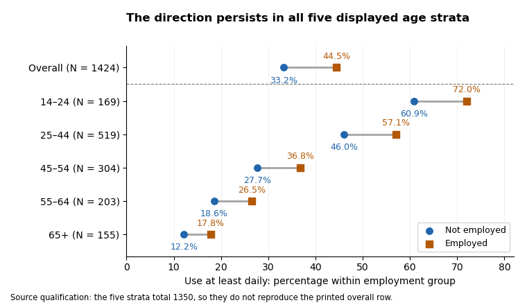
At-least-daily use is more common among employed respondents in each displayed age stratum; the printed overall row is a separate, non-reconciling input
. Details. 
Across the visible strata, frequent use declines strongly with age in both employment groups, while the at-least-daily employment difference remains positive. This is compatible with age being important to the use distribution and with a positive employment association persisting after age stratification. It is not a demonstrated Simpson's paradox: none of these displayed threshold differences reverses direction. The evidence also does not establish how much age confounds the overall result, because the strata do not reproduce its sample and the oldest age labels disagree across figures. Among young respondents the positive ordinal association coexists with a reversed never-use contrast, so the threshold summary should not be described as stochastic domination of every conditional distribution.
Ordinal measures summarize a different aspect from the omnibus tests. Counting pairs from each visible table gives Goodman and Kruskal's gamma approximately in age order. For use as response, the corresponding Somers' D values are about ; Kendall's tau-b values are ; and Stuart's tau-c values are . They are all positive and modest, but not interchangeable. Gamma discards pairs tied on either variable; Somers' D includes response ties separated by employment; Kendall's tau-b adjusts for ties in both variables; Stuart's tau-c adjusts for table dimensions. The printed second-variable tie counts violate the unordered-pair partition for ordinal data in all five strata, so the printed Somers and tau-b values should not be accepted as independently verified numbers.[ref]
Ordinal association measures in the DescTools documentation. KendallTauB and StuartTauC: distinct tie/table-size adjustments
Goodman and Kruskal's lambda for predicting the use category from employment is zero in all five visible strata: each employment row has the same modal use category as its stratum overall. This does not contradict their nonzero gamma or V, because the rest of each category distribution can change without its mode changing. Reversing the prediction target gives about for predicting employment from use. In the original display these are the second lambda values; identify the target directly rather than relying on ambiguous row/column-dependent labels. The contingency coefficient, another unsigned transformation of the Pearson statistic, adds no new direction and cannot repair a corrupted test statistic.
Even if all printed p-values were trusted, a significant result in one age group and a nonsignificant result in another would not prove that their effects differ. A statistical interaction needs a direct comparison of effects on a specified scale, not a comparison of significance labels. Five separate tests also create a multiple-testing issue if the aim is to claim at least one association; choosing categories or a threshold after inspection adds further selection. A joint conditional independence test for stratified contingency tables or an appropriate categorical-response model can target a clear combined hypothesis, with exact or simulation-based calibration where needed. Such a model would require coherent input tables before it could resolve the source discrepancies. The sound conclusion is a consistent positive descriptive tendency within the five shown strata, with no count-supported nominal 5% omnibus rejection in an individual stratum, and insufficient coherent output for a claimed causal or precisely quantified age-adjusted effect.
Read conditionally, the fitted slope says that a one-point higher skill score is associated with about 0.209 more household devices in the fitted conditional expectation. The printed summary also claims a significant slope and about 28.93% explained sample variation. Those claims cannot be assembled into one valid fitted model: several regression identities fail, so a single verified coefficient-and-uncertainty report is unavailable.
The response is a device count, while the predictor is a skill score. A simple linear regression models , where is the device count and the skill score. Ordinary least squares chooses the intercept and regression slope to minimize the residual sum of squares. The regression slope describes a conditional association, not the causal effect of training or acquiring a device.
The descriptive statistics put the device count between and , with sample mean about and sample standard deviation about among records. Skill scores range from to , with sample mean about and sample standard deviation about among records. Two missing skill values account for the stated two deleted records; because device counts have no missing values, the regression complete-case sample has observations. Estimating two regression coefficients leaves residual statistical degrees of freedom, matching that part of the output. The units of the two standard deviations differ, so comparing with does not establish that skill is more variable in a substantive sense.
If the coefficient estimates are trusted, the fitted values follow . The intercept predicts about devices at a skill score of zero; zero is within the stated score range, but precision and the number of observations near zero are not shown. A five-point increase in score corresponds to about additional fitted devices and a ten-point increase to about . At a score of ten the fitted value is about , and at 24 it is about . Expected counts may be fractional even though individual counts are integers. These are conditional interpretations of the coefficient fields, not reconstructed raw observations or validated individual predictions.
A coefficient's standard error estimates its sampling uncertainty, whereas the residual standard error describes unexplained response variation. For the intercept, , agreeing with the printed and rounded . Conditional on the model assumptions, this would reject a zero intercept at conventional significance levels. The intercept test is not a test of whether skills predict devices. For the slope, the printed would reject at 5% but not 1%; it does not assign a probability to the null hypothesis or measure the usefulness of prediction. The significance stars simply encode thresholds and add no independent evidence.[ref]
Summarizing Linear Model Fits in the R documentation. Value: coefficient, standard-error, two-sided t and p columns; sigma, residual degrees of freedom and F statistic
The slope row fails its own arithmetic check:At statistical degrees of freedom the ratio gives a two-sided p-value about , while the printed gives about ; neither is . Thus the choice of which source field is trusted changes the apparent strength of evidence, including the 1% decision. A 95% confidence interval built conditionally from the printed estimate and standard error would be about , but it is not a verified interval from a coherent fitted model. In fact, using the printed residual standard error , the complete predictor sample size and predictor standard deviation gives a slope standard error near , not .
The printed coefficient of determination would mean that the fitted line explains of the complete-case sample's centred device-count sum of squares relative to an intercept-only fit; remains unexplained by that comparison. It is not the percentage of devices caused by skill, the fraction of correctly predicted households, or a measure of future predictive accuracy. The adjusted coefficient of determination is consistent with that and the given sample size, allowing rounding. The small adjustment reflects fitting one slope among many cases; it does not validate the model.
For a one-predictor ordinary least squares fit with an intercept and the usual common-variance standard errors, the simple-regression output identities requireHere the printed slope t gives , the printed F field says , and the printed instead implies . These cannot all hold. Moreover, on and statistical degrees of freedom has p-value about , not . Reading the printed F p-value alone would give a 1% significant test of the zero-slope model, but its reported calibration is incompatible with its statistic. No significance label resolves these identities.
There is also a contradiction that does not depend on tail probabilities. Ordinary least squares with an intercept makes the arithmetic mean of fitted values equal the arithmetic mean of observed responses on the analysed records. The printed coefficients and predictor mean give . Deleting two device counts anywhere in the printed range , and allowing the reported overall mean to be rounded, would leave the complete-case device mean between approximately and . The mean bounds after deleting bounded observations therefore rule out reconciling with the response summary merely by citing those two missing predictor values. This is not the mistaken assumption that full-sample and complete-case sample means must always be identical.
If its own field were trusted, residual standard error estimates the unexplained response standard deviation, in device-count units. It is neither the standard error of the slope nor a guarantee that every prediction is accurate to devices. The residual five-number summary has extremes near and and median near , with central quartiles near and . The roughly central median does not establish normally distributed errors, homoscedasticity, independence or a linear conditional expectation. A residual-versus-fitted plot could check curvature and spread; a normal probability plot could assess an error-shape approximation. Neither diagnostic can be recovered from five residual quantiles alone. Individual prediction intervals include response variation as well as coefficient uncertainty and are wider than confidence intervals for the conditional expectation.
For conventional finite-sample t and F calibration, a normal linear model assumes independent mean-zero normal errors of common variance with an appropriate predictor specification. Mean-zero errors conditional on skill and adequate sampling remain essential even when large-sample approximations relax normality. A bounded count response can have nonconstant conditional variance, so residual diagnostics and a scientifically suitable response model matter; count data do not become normally distributed just because the sample is large. Poisson regression is one possible alternative to investigate, but its own conditional mean–variance assumptions and the bounded device range require assessment, not automatic substitution. Complete-case selection can also bias the fitted association if it depends on the response in a relevant way. The only safe summary is conditional: the printed slope is positive, but the numerical effect, its standard error, t/F evidence and explanatory fit require a corrected, coherent output before a single definitive regression claim is made.
Solutions to all six questions of the 12 December 2019 Statistics Core examination. Oxford examination release ZIP, member
Digital Social Research Statistics Core/2019 Michaelmas a14564w1.pdf. All seven numbered figures and the unnumbered output for Question 1 are available. The printed group means and overall mean in Question 1 cannot describe one complete sample; that inconsistency is kept explicit. Calculations below use the supplied summaries and counts, without inventing individual records.Conditional on the printed two-group test output, the male-coded group has higher mean efficacy by about 1.034 scale points, with a 95% confidence interval of about 0.785 to 1.282 points. This is strong evidence against equal population means under the test's assumptions. It does not establish a causal effect, and the accompanying overall mean is inconsistent with the group summaries.
Here the coding identifies group 0 as male and group 1 as female in this dataset. The counts are 1215 and 1251, respectively, or approximately 49.27% and 50.73% of 2466 observations. These are sample compositions, not evidence that the sample represents every population of interest. The continuous efficacy scale runs from 0 to 16, with higher scores indicating stronger efficacy. Its printed sample median is 10 and its quartiles are 8 and 12, so its interquartile range is 4 points. The printed overall sample mean, 9.348, requires the separate consistency qualification below.
Let and denote the two population means. The null hypothesis is , and the alternative hypothesis is the two-sided test . The two sample means giveThe positive sign means higher mean efficacy in group 0, given this coding; it does not say that every member of that group has higher efficacy than every member of group 1.
Welch's t-test estimates uncertainty from the two groups separately rather than assuming equal population variances:The printed implies a standard error of approximately points. The noninteger 2277.4 statistical degrees of freedom comes from the Welch approximation; it is not a count of fractional observations. Using the corresponding Student t-distribution gives the displayed p-value, approximately . The test and interval calculations agree to the precision of the printed numbers.[ref]
Student's t-Test in the R documentation. Arguments and Details: two-sided default and unequal-variance Welch calculation; Value: estimates, statistic, degrees of freedom and interval
A p-value is the probability, under the null hypothesis and the assumed sampling model, of a test result at least as incompatible with equal means as the observed result. It is not the probability that the null hypothesis is true, the probability that the finding is a chance mistake, or the size of the mean difference. At a prespecified significance level such as , this result rejects the equal-mean null hypothesis; it also rejects at 1%. A Type I error is rejection when that hypothesis is true, and a valid level- procedure controls its long-run probability. A Type II error is failure to reject a false hypothesis; statistical power is the probability of rejection under a specified alternative. Neither error probability for this one realized claim is supplied by its p-value.
The 95% confidence interval comes from , with critical value about 1.961. Its positive endpoints support the same direction and exclude zero. The frequentist 95% statement concerns coverage over repeated samples, not a 95% posterior probability assigned to this fixed interval. Reporting the difference in scale points supplies an effect size; its practical importance also depends on what a point means substantively. A very small p-value alone does not answer that question.
The inferential calculation requires independent observations and an appropriate sampling model. With these large groups, approximately normal sampling distributions of the means can be more plausible than normality of individual bounded scores, but a large sample size does not correct dependence, clustering, selection bias or measurement problems. The output does not establish random assignment or remove possible confounding, so the estimated difference is an association.
There is a material source inconsistency. For exhaustive groups with complete outcome data, the sample mean must be the sample-size-weighted mean of the group means:which cannot round to 9.348. Figure 7 independently reports all 2466 efficacy values present and again gives 9.348; Question 6 refers back to the same continuous scale. The pooled-mean compatibility under rounding rules out explaining the discrepancy by the displayed decimal precision. Thus the two-group test supports the stated conclusion if its own group summaries and test fields are trusted, while the overall mean cannot simultaneously be accepted as a coherent summary of those groups. No unprinted exclusion or uniquely correct replacement mean is established.
All three frequency tables describe 2466 valid observations with no reported missing values. The sample is overwhelmingly White, Medium is the most common efficacy category, and disagreement with the technology-failure statement is more common than agreement. These statements describe the sample rather than establish population composition or causal relationships.
In a frequency table, a count gives the number of observations in a category, and a percentage divides that count by the full sample total. A valid percentage instead uses the total with an observed value of that variable. Here the two denominators coincide because every table reports zero missing values. A cumulative percentage adds categories in the displayed order; its substantive meaning depends on whether that order is meaningful.
The ethnicity counts are 77 Asian, 57 Black and 2332 White respondents, or 3.12%, 2.31% and 94.57%. Ethnicity is a nominal categorical variable: the displayed order is not a low-to-high ethnic scale. Its cumulative percentages are bookkeeping for that listing rather than an interpretable ranking. The two minority groups are small relative to the White group, which will matter for the precision and expected cell counts of the stratified comparisons.
For the three-category efficacy measure, 908 observations are High, 972 Medium and 586 Low, giving 36.82%, 39.42% and 23.76%. Medium is the mode, and 76.24% fall in the combined High-or-Medium categories. This is an ordinal categorical variable, but the table does not imply equal numerical distances between categories. Its order is descending efficacy, High then Medium then Low. Therefore the cumulative 76.24% refers to that upper portion of the scale, not to the proportion at or below Medium under an ascending convention. The cutpoints used to form these categories are not supplied and need not be invented to interpret their frequencies.
For
techfail_chr, 336 strongly disagree, 922 disagree, 490 are neutral and 718 agree: 13.63%, 37.39%, 19.87% and 29.12%. The wording concerns not trusting technology because it fails when needed. Thus moving toward Agree means more distrust, not more trust. Combining the two disagreement categories gives , versus 29.12% agreement and 19.87% neutrality. Adding the separately rounded displayed percentages gives 51.02%; the difference is ordinary rounding error. There is no displayed strongly-agree category, so its frequency cannot be inferred or added to the agreement count.The technology percentages add to 100.01%, including the printed valid-total figure. The integer counts still sum exactly to 2466; rounded percentages need not sum exactly to 100%. Finally, three separate univariate frequency tables say nothing by themselves about which efficacy categories the trusting or distrusting respondents occupy. That requires the joint information in the later contingency tables.
Greater technology distrust is associated with lower efficacy in the overall sample. The omnibus evidence against independence is strong, while the unsigned association magnitude is modest: on 6 statistical degrees of freedom, and Cramér's V about 0.148. The observational study does not establish that changing trust would cause efficacy to change.
Rows identify the technology response and columns identify efficacy. Each body percentage is a within-row conditional probability estimate, not a column percentage. For example, of those who strongly disagree with the distrust statement have High efficacy, whereas of those who agree do. The difference is about 21.69 percentage points. High efficacy decreases across all four rows: 49.40%, 42.41%, 31.02%, 27.72%. Low efficacy is 20.54% in the strongly-disagree row, 18.00% in Disagree, 21.43% in Neutral and 34.26% in Agree. Thus the overall pattern is clear without claiming that every category changes monotonically: the low-efficacy proportion initially falls, and the Medium proportion peaks at 47.55% among neutral respondents.
For the Pearson chi-squared test of independence, the null hypothesis says that the two categorical variables are independent, equivalently that the efficacy distribution is the same in every technology-response row. With row totals and column totals , the expected frequency under that hypothesis is , andAll twelve expected frequencies exceed 79, with minimum about 79.844, so sparse expected cells are not the concern here. Under independent sampling and the usual large-sample calibration, the very small p-value rejects independence at conventional significance levels. This is an omnibus finding: it does not provide a separate adjusted significance test for every pair of row percentages.[ref]
Pearson's Chi-squared Test for Count Data in the R documentation. Details: product-marginal null hypothesis and asymptotic chi-squared calibration
The likelihood-ratio test of independence in a contingency table uses . The supplied with 6 statistical degrees of freedom gives . Its displayed 0.000 is rounded, not an exact zero. It corroborates the omnibus finding. The generalized phi coefficient is , the contingency coefficient is about 0.205, and Cramér's V is . These are unsigned measures of association strength rather than three additional significance tests; they do not describe causal effects or percentages of variance explained. Their magnitude and the small p-value answer different questions, especially with a large sample size.
The ordinal measures use the displayed order: increasing row index means increasing distrust, while increasing column index means decreasing efficacy. There are 882033 concordant pairs and 552543 discordant pairs. Hence Goodman and Kruskal's gamma isIts positive sign therefore means that increasing distrust tends to accompany movement toward lower efficacy. Under an ascending efficacy order its sign would be negative, by sign reversal under reversal of one ordinal ordering. Goodman and Kruskal's gamma ignores tied pairs; it is not a claim that 23% of efficacy variation is explained. The displayed pair counts partition all unordered pairs correctly, including ties. Somers' D for efficacy given technology is about 0.151, Kendall's tau-b about 0.158, and Stuart's tau-c about 0.163. Their different denominators handle ties or table dimensions differently, so their differing magnitudes do not constitute disagreement about the direction.[ref]
DescTools documentation for gamma, Somers' D and lambda. GoodmanKruskalGamma and SomersDelta, Details: tied-pair exclusions and the directional denominator
[ref]Ordinal association measures in the DescTools documentation. KendallTauB and StuartTauC: tie and table-size adjustments
Goodman and Kruskal's lambda concerns the proportional reduction in errors when predicting a most frequent category, not ordinal movement. Without technology information the modal efficacy category is Medium, producing errors. Choosing a separate modal efficacy category in each technology row yields errors. Thus . In the reverse prediction direction the reduction is , matching the other printed lambda. The improvement in modal classification is small even though independence is decisively rejected. Both the conditional percentages and these distinct summaries support a real sample association; ethnicity and other possible confounders still require attention before any causal account.
There are descriptive ethnic differences in the distribution of technology distrust, but the omnibus evidence is borderline and the unsigned association is small. The printed Pearson test just rejects independence at 5%, while the likelihood-ratio test does not; neither establishes a strong ethnic pattern or a causal effect.
Read the body percentages within each ethnic group. Strong disagreement with the distrust statement occurs among 24.68% of Asian respondents, 10.53% of Black respondents and 13.34% of White respondents. Agreement occurs among 27.27%, 21.05% and 29.37%, respectively. Neutral responses are 20.78%, 26.32% and 19.68%. Thus Asian respondents are especially likely to be in the strongly-disagree category, while Black respondents have the largest neutral share. The mode for Black and White respondents is Disagree; Asian respondents have a tie between Disagree and Agree at 21 observations each. The small group totals, 77 and 57, mean that a few observations can materially change the minority-group percentages.
The Pearson chi-squared test of independence has , statistical degrees of freedom and . Under its sampling assumptions, this is a nominal rejection at a prespecified 5% significance level, but not at 1%. The minimum expected frequency is about 7.766, so this particular table has no expected cell below five. The alternative likelihood-ratio test of independence in a contingency table gives and , printed as 0.074. These are different test statistics, not contradictory versions of the same calculation. Their different threshold decisions show that the evidence is close enough to the conventional boundary to warrant qualification rather than selection of the more favourable label.
The generalized phi coefficient is about 0.071, the contingency coefficient about 0.071 and Cramér's V about 0.051. They indicate a small overall unsigned association. This does not erase the particular descriptive percentage differences, and a small p-value is not a measure of their substantive size. Conversely, failure of the likelihood-ratio test to reject at 5% is not evidence that every ethnic group has exactly the same population response distribution.
Ethnicity is a nominal categorical variable, with no natural rank Asian–Black–White. Therefore the printed Goodman and Kruskal's gamma of 0.079, Somers' D of 0.058, Kendall's tau-b of 0.022 and Stuart's tau-c of 0.009 have no invariant substantive ordinal interpretation here. Permuting the ethnicity labels can change the ordinal pair comparisons without changing the underlying observations or their nominal association. These values are not evidence for an ethnic hierarchy; Cramér's V and the actual within-group percentages are appropriate summaries for this question.[ref]
DescTools documentation for gamma, Somers' D and lambda. GoodmanKruskalGamma and SomersDelta, Details: ordinal-scale requirement
Both directional values of Goodman and Kruskal's lambda are zero. Knowing ethnicity does not improve the number of correct modal predictions of technology response: Disagree remains a modal category within every ethnic group, including the Asian tie. In the reverse direction, White is the most frequent ethnicity within every technology-response column, so knowing technology does not improve modal ethnicity predictions either. Zero lambda therefore coexists with unequal conditional distributions and a nonzero Pearson chi-squared statistic; modal prediction discards changes that do not change the most frequent category. The supported conclusion is a small, weakly evidenced nominal association, with its descriptive pattern and uncertainty stated explicitly.
The White stratum retains the overall distrust–lower-efficacy pattern, the Asian stratum shows a stronger but irregular version of it, and the Black stratum has an opposite descriptive ordinal direction. This supports replication in the dominant stratum together with possible specification by ethnicity in the elaboration model. Sparse minority tables and different significance labels do not by themselves establish a population statistical interaction.
Each table fixes ethnicity and compares the efficacy conditional distributions across technology responses. The body percentages use the technology-response row total within that stratum. The same labels, coding direction and efficacy order apply as before. The strata contain 77, 57 and 2332 observations; they sum to 2466 and their cells reproduce the overall table exactly. Consequently the comparison is genuinely a stratification of the supplied overall counts, rather than a comparison of unrelated samples.
For Asian respondents, High efficacy is 78.95% among those who strongly disagree with the distrust statement, falling to 23.81% among those who disagree, 18.75% among neutral respondents and 19.05% among those who agree. The strong-disagreement versus agreement contrast is about 59.90 percentage points, based on 15 of 19 versus 4 of 21 respondents. This is a large descriptive contrast, but the rest of the table is not a simple monotone progression: Low efficacy peaks at 47.62% in Disagree, versus 10.53% in Strongly disagree, 18.75% in Neutral and 23.81% in Agree; Medium efficacy exceeds 57% in the last two rows. The striking first row is part of a more irregular categorical pattern.
The Asian Pearson chi-squared test of independence gives , 6 statistical degrees of freedom, . The likelihood-ratio test gives , ; its displayed 0.000 is a rounding convention. Cramér's V is about 0.430, compared with 0.148 overall. The generalized phi coefficient is 0.608 and the contingency coefficient 0.519. Two of twelve expected frequencies are below five, with minimum 4.156. This is a modest sparse-cell warning rather than a reason to delete the observed cells, but asymptotic calibration should still be qualified and could be checked by an exact or fixed-margin Monte Carlo test.
The Asian Goodman and Kruskal's gamma is about 0.323, from 1025 concordances and 524 discordances, so its displayed-order direction agrees with the overall association. Somers' D for efficacy given technology is about 0.226, Kendall's tau-b 0.241 and Stuart's tau-c 0.253. These stronger ordinal summaries do not imply that every individual row transition is monotone. Goodman and Kruskal's lambda is about 0.362 for predicting efficacy from technology and 0.286 in the reverse direction: the technology row changes the modal efficacy prediction sufficiently to reduce its errors by about 36.2%. This is a reduction in modal-classification errors, not a fraction of efficacy variance explained.
For Black respondents, High efficacy is 0 of 6, or 0%, in Strongly disagree; 8 of 24, or 33.33%, in Disagree; 2 of 15, or 13.33%, in Neutral; and 7 of 12, or 58.33%, in Agree. Low efficacy is 16.67%, 25.00%, 20.00% and 8.33%, respectively. The strongest-disagreement versus agreement High-efficacy contrast is therefore percentage points, opposite to the Asian and White contrasts. The zero observed High count in the first row does not prove zero population probability, especially with only six respondents in that row. These percentages are compatible with a reversed tendency, but considerable sampling uncertainty is unavoidable.
The Black Pearson chi-squared test of independence gives , 6 statistical degrees of freedom and . The likelihood-ratio test gives , , also above 5%. Thus neither nominal test rejects at 5%; this does not establish exact independence. Eight of twelve expected frequencies are below five, with minimum about 1.158, making the usual large-sample calibration particularly questionable. An exact conditional analysis or Monte Carlo test would be more defensible for a calibrated inferential claim; no uncomputed simulated p-value is asserted.[ref]
Pearson's Chi-squared Test for Count Data in the R documentation. Details: fixed-margin sampling for simulated contingency-table tests
The Black Cramér's V is about 0.308, the generalized phi coefficient 0.435 and the contingency coefficient 0.399. An unsigned magnitude of this size can coexist with a nonsignificant test in a small sample. There are 254 concordances and 457 discordances, giving Goodman and Kruskal's gamma about , Somers' D about , Kendall's tau-b about and Stuart's tau-c about . Their negative signs agree with the reversed displayed-order direction. Goodman and Kruskal's lambda is about 0.107 for efficacy given technology and zero for technology given efficacy. In the latter direction, Disagree remains a modal technology category within every efficacy column, so modal prediction gains nothing despite the changed conditional percentages.
For White respondents, High efficacy decreases from 48.55% in Strongly disagree through 43.10% and 32.03% to 27.45% in Agree. The extreme-row contrast is about 21.11 percentage points, from 151 of 311 versus 188 of 685. Low efficacy is 21.22%, 17.10%, 21.57% and 35.04%, respectively. This closely resembles the overall distribution, including the fact that the Low category is not monotone at every step. The White Pearson chi-squared test of independence gives , 6 statistical degrees of freedom and ; the likelihood-ratio test gives , . All expected frequencies exceed 74, so sparse cells are not the problem for these nominal tests.
The White Cramér's V is about 0.152, the generalized phi coefficient 0.215 and the contingency coefficient 0.210. Goodman and Kruskal's gamma is about 0.236, Somers' D 0.155, Kendall's tau-b 0.162 and Stuart's tau-c 0.167: close to the overall ordinal summaries and in the same direction. The two values of Goodman and Kruskal's lambda are about 0.061 for efficacy given technology and 0.062 for technology given efficacy. They again indicate only a small improvement in modal prediction. The large sample size helps explain why the White test has a much smaller p-value than the smaller strata, without implying that its association magnitude is the largest.
The original figure below plots selected empirical conditional probabilities from all the cells. It gives the opposite small-stratum pattern and the dominant White pattern a common scale; it is not a reproduction of a source figure, an estimated continuous trend or a display of uncertainty intervals.
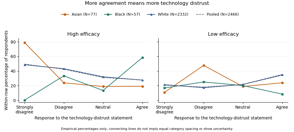
Efficacy distributions across technology-distrust responses: contrasting ethnic strata and the pooled sample. Lines only connect the four ordered categories; group sizes and sparse cells limit inference.
Details. 
The elaboration model asks how the original association changes when a third variable is held fixed. If the association disappeared throughout the strata, an explanation by the control variable might be plausible, subject to a credible causal ordering. Here it persists in the White group, which supplies 94.57% of the sample, and is stronger on several descriptive measures in the Asian group. Therefore ethnicity does not simply explain away the relationship. The White result is a replication of the broad pattern; the reversed Black direction and the Asian shape suggest descriptive specification or possible effect modification. The output supplies no temporal or causal design that would distinguish an actual causal mechanism from other confounding, measurement differences or sampling variation. It also does not demonstrate a Simpson's paradox in which the association reverses in every stratum: that is not what the displayed tables show.
The predominance of White respondents explains why the pooled pattern resembles theirs. By the law of total probability, each technology row's efficacy distribution is a mixture over ethnicity, using the ethnic proportions within that technology row. Those weights need not equal the overall ethnic proportions. As an optional descriptive comparison, standardization with common weights using the overall ethnic shares gives High-efficacy proportions of about 48.38% in Strongly disagree and 27.90% in Agree, a 20.48-percentage point contrast, compared with the crude 21.69-point contrast. This explicitly defined adjustment leaves the broad contrast intact; it is not a causal estimate and does not turn the three different stratum patterns into one common effect.
Finally, a significant test in one group and a nonsignificant test in another is not itself a test that the groups' associations differ. A formal statistical interaction requires a directly specified heterogeneity test or model on a chosen effect scale. The omnibus tests also address whole categorical distributions, whereas gamma and the High-efficacy contrast describe particular ordered features. Multiple stratum tests create a multiple testing issue if used to select a discovery. The defensible result is an association that survives stratification in the dominant group, with important descriptive heterogeneity that merits a direct, sparse-cell-aware investigation rather than an assertion that ethnicity causes the difference.
The fitted age slope is very small and negative, about efficacy points per year, with no conventional evidence against a zero linear slope: , . The model explains only about 0.0367% of the observed efficacy variation. These results concern a linear association, not proof of no possible age relationship or a causal effect of ageing.
The descriptive statistics report 2466 observed ages and efficacy scores, with no missing values for either variable. Age ranges from 14 to 97 years, with sample mean 52.689 years and sample standard deviation 19.064 years. Efficacy ranges from 0 to 16, with sample mean 9.348 and sample standard deviation 3.176 scale points. The standard deviations use different units and should not be compared as though their numerical ratio measured relative substantive variability. The efficacy mean retains the conflict with Question 1's group summaries; that conflict is not resolved by this separate regression output.
A simple linear regression models , where is efficacy and is age in years. Ordinary least squares chooses the coefficients to minimize the residual sum of squares. From the printed coefficients the fitted line isHolding to this model, ten additional years correspond to fitted scale points. For example, the fitted mean is about 9.453 at age 20 and 9.261 at age 80, a difference of about points. These are fitted means, not exact predictions of individual scores. The line does not imply that every person's efficacy falls at that rate, nor that cross-sectional age differences identify within-person changes over time.
The intercept is the predicted mean at age zero, about 9.517. Since zero is outside the observed 14–97 age range, its direct interpretation requires extrapolation. The printed standard error of 0.188043 and yield the extremely small displayed p-value for a zero intercept. That test does not test whether age is a useful predictor. Recentring age at its observed sample mean would put the intercept near , the fitted mean at a substantively relevant reference age. This agrees with the rounded overall efficacy mean.
The age standard error is 0.003356 points per year. The coefficient divided by this standard error gives , agreeing with the printed t value. Estimating an intercept and one regression slope from 2466 observations leaves residual statistical degrees of freedom. Under a correctly specified normal linear model, the Student t-distribution provides the stated two-sided p-value. At 5%, or 1%, it does not reject . The p-value is not a 34.2% probability that age has no effect, and nonrejection does not establish a practically negligible effect size.[ref]
Summarizing Linear Model Fits in the R documentation. Value: coefficient estimate, standard error, two-sided t and p columns; residual degrees of freedom
A 95% confidence interval calculated from the printed estimate and standard error is approximatelyor about points per decade. It includes zero and gives the scale of slopes compatible with these summaries and assumptions. Assessing a practically negligible effect would require an explicit substantive tolerance and an appropriate equivalence test, not simply the fact that . A nonlinear association could also coexist with a near-zero overall linear slope.
The coefficient of determination is , meaning that the fitted line explains about of the sample's centred efficacy sum of squares compared with an intercept-only fit. This is not 36.7%, a fraction of people whose efficacy is predicted correctly, or the proportion of efficacy caused by age. The adjusted coefficient of determination, approximately , is slightly negative because its penalty for estimating the extra coefficient exceeds the tiny improvement in fit. It need not be constrained to be nonnegative and does not mean a negative amount of explained variation.
The overall on 1 and 2464 statistical degrees of freedom, with , tests the same zero-slope hypothesis as the age t test because there is only one predictor. The simple-regression output identities give and ; the printed numbers agree allowing their displayed precision. The signed Pearson correlation coefficient is consequently about . These are related summaries of the same weak linear association, not independent corroborating tests.
The residual standard error of 3.177 points estimates the typical unexplained error scale under the fitted model. It is close to the efficacy sample standard deviation, as expected when the line explains almost none of the variation. It is not a standard error of the slope or a guarantee that each individual's prediction error lies within 3.177 points. The residual summary spans roughly to , with sample median about 0.573 and central quartiles about and . An ordinary least-squares fit with an intercept has zero mean residual, not necessarily zero median residual. These few quantiles cannot establish normality, constant conditional spread, absence of outliers or linearity. The apparent last-decimal discrepancies among rounded error scales and other summary fields do not force an additional contradiction: their rounding intervals admit compatible regression summaries.
The conventional uncertainty calculations assume independent, mean-zero errors conditional on age, an appropriate linear mean, and homoscedasticity; normal errors give the usual exact finite-sample t and F calibration. Large samples can relax some distributional requirements but do not remove confounding, selection bias or dependence. A residual-versus-fitted plot could reveal curvature or changing spread, and a normal probability plot could assess error shape; neither plot can be reconstructed from the printed residual quantiles. A prediction interval for an individual includes residual variation and is wider than a confidence interval for the mean response. The supplied output supports a very weak, imprecisely signed linear association with little predictive gain from age alone, while leaving nonlinear, causal and design-based questions unresolved.
Articles by others on the same topic
There are currently no matching articles.