Past exam of the laser science and quantum information processing course of the University of Oxford / 2017 / 2

Measure the phase relative to propagation through the same geometrical thickness of air. If the lens's central thickness is $t_0$, its spherical surface givesThe optical-path excess is $(n-1)t(x)$, so the phase imparted by the lens isThe constant part is a spatially uniform phase. The physically important lens transmission is therefore $T_f(x)=\exp [-ik{x}^2/(2f)]$ withOne way to identify the focus is to append propagation to the on-axis point a distance $f$ away. Its path phase has the paraxial contribution $+k{x}^2/(2f)$, which cancels the lens phase. Thus all incident portions of a plane wave add with the same phase at that point. The diagram below shows the thickness change and both Fourier-transform arrangements.

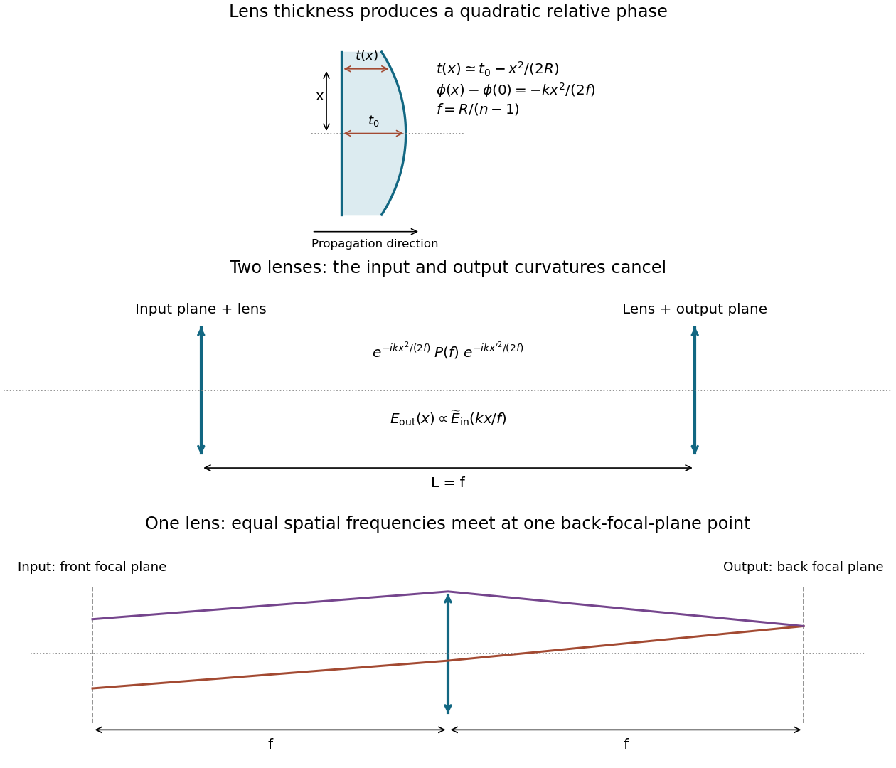
Apply the first lens, propagate, and apply the second lens. Omitting only common prefactors and uniform phases,The coefficients of both $x^2$ and $x^{\prime 2}$ vanish if and only if $f=L$. The remaining cross term is $-ikx{x}^{\prime }/L$, soThe Fourier convention here is $\tilde{E}(q)=\int e^{-iqx}E(x)dx$. Finite clear apertures would truncate the field and limit the spatial-frequency range; the ideal relation assumes the paraxial field fits within both lenses.

Free propagation is convolution with a chirp, $K_L(x)=C_L{e}^{ikL}{e}^{ik{x}^2/(2L)}$. The convolution theorem therefore turns it into multiplication by its Fourier transform. Complete the square:The Gaussian integral then givesThus the wavevector-dependent phase isup to an overall phase convention; after removing the carrier it is $-L{k}_{\perp }^2/(2k)$. This also follows from $k_z=\sqrt{k^2-k_{\perp }^2}\simeq k-k_{\perp }^2/(2k)$.

Normalization qualification: the source keeps a two-dimensional-style prefactor while integrating over only one transverse coordinate. With its literal $C_L=ik/(2\pi L)$, there is an additional $q$-independent factor, rather than solely a unit-modulus multiplier. A properly normalized one-dimensional Fresnel propagator has $C_L=\sqrt{k/(2\pi iL)}$, which cancels the square-root factor above and makes propagation a pure Fourier-domain phase. For example, the literal source kernel multiplies a plane-wave Fourier mode by a factor of magnitude $\sqrt{k/(2\pi L)}$, not one. The spatially dependent phase and the proportional Fourier-transform results remain unchanged. ^[ref]

Place the input plane one focal length before a single positive lens and the output plane one focal length after it. The lens maps each incident transverse spatial frequency to its corresponding point in the back focal plane. Referencing the input to the front focal plane removes the otherwise present output phase curvature, giving an exact scaled Fourier transform within the same paraxial model.

A short ray-matrix check makes the geometry explicit. With free propagation $P(f)$ and lens matrix $L(f)$,The vanishing diagonal entries are the Fourier-plane condition; the output is proportional to ${\tilde{E}}_{\mathrm{in}}(kx/f)$. The final panel of the original diagram in part a shows the two focal distances. A lens with input immediately on its surface and output at the back focal plane would generally leave a quadratic output phase; the front-focal-plane choice avoids it.