Source paper: www.whatdotheyknow.com/request/oxford_physics_past_papers_2/response/2340696/attach/5/Physics%20Papers%202016.pdf?cookie_passthrough=1. The cover dates this paper to Trinity Term 2017, 14 June; the bundle's 2016 filename does not determine its year. The four marked requests in each question are scoped a–d below. Computational-basis vectors use left-to-right qubit order unless another order is explicitly stated.
A laser relaxation oscillation is the damped exchange between stored upper-level excitation and intracavity photon number after a small perturbation of a lasing steady state. Extra photons increase stimulated depletion of the upper level; the resulting smaller gain then reduces the photon population. Pumping subsequently replenishes the inversion, so the two populations overshoot their equilibrium values before damping settles them.
Laser spiking is the corresponding large-signal sequence of intense output pulses, often during switch-on. Excitation first accumulates while the optical field is small. Once gain exceeds loss, rapid stimulated emission releases this stored energy in a spike, depleting the inversion below threshold. Recovery can produce further spikes. This is distinct from an externally imposed Q-switching cycle, although both draw on stored excitation.
Many solid-state gain media have upper-state lifetimes far longer than the cavity photon lifetime. The optical polarization relaxes rapidly, leaving the two slow rate-equation variables of a class-B laser. A long-lived population reservoir and a much faster photon response make underdamped recovery and pronounced startup spiking common. The criterion and frequency follow from the linearization in part c; they are not universal consequences of the word “solid-state”.
Let be the light's group velocity in the fibre, with unit mode overlap and a uniform transverse mode area. The fibre-laser gain-volume rate equations follow because the upper-level density is defined per doped volume, whereas the photon density is defined per full cavity volume. Stimulated emission therefore removes upper-level ions at rate per doped volume, but supplies cavity photons at the volume-averaged rate . ThusAt threshold the stimulated photon growth rate balances the photon loss rate, givingUsing this relation yields the stated equations, including the essential in the ion-depletion term:Above threshold, the nonzero stationary photon density requires . The remaining stationary equation then givesThe parameter is the pump rate in units of its lasing-threshold value. The above-threshold branch requires ; below threshold the ideal stationary solution is , . Spontaneous emission into the lasing mode has been omitted in this deterministic model, so an exactly zero initial field would need a seed or noise to start, even when the zero-field branch is unstable.
Write and . Keeping terms linear in the perturbations givesEquivalently,The characteristic exponents areConsequently the above-threshold steady state has damped oscillations precisely whenTheir ordinary frequency isThe approximation neglects the damping correction when . The exponential envelope decays on time . The doped-volume fraction cancels out of this linear frequency once the pump is expressed through . [ref]
https://ocw.mit.edu/courses/6-974-fundamentals-of-photonics-quantum-electronics-spring-2006/18f30fad63a62ef4dd894d3752b55a60_chapter7.pdf. MIT 6.974, Chapter 7, laser dynamics and relaxation oscillations
The upper-state density is clamped near threshold once the laser operates, so excess pumping mainly increases photon density and output power. For approximately pump-independent absorption efficiency, , and both and should rise approximately linearly with .
The left ordinate is the square of the frequency, in , rather than frequency in kHz. Reading the original triangles gives a threshold near – and a slope about . A representative straight-line fit to visually read marker centers gives and . ThereforeThe displayed precision is limited by graph reading and scatter; a lifetime around is the meaningful result. The output squares have a compatible threshold and an approximately constant slope above it.
The round-trip time isIf mirror transmission is the only appreciable passive loss, energy decays by per round trip. For ,a power reflectance of roughly 65%. The exact exponential is preferable to replacing by , since the inferred round-trip loss is not tiny. If distributed fibre loss is appreciable, the lifetime instead fixes the total round-trip retention; without a separate loss measurement, the bare mirror reflectance is not uniquely determined and is at least this retention factor.
Measure the phase relative to propagation through the same geometrical thickness of air. If the lens's central thickness is , its spherical surface givesThe optical-path excess is , so the phase imparted by the lens isThe constant part is a spatially uniform phase. The physically important lens transmission is therefore withOne way to identify the focus is to append propagation to the on-axis point a distance away. Its path phase has the paraxial contribution , which cancels the lens phase. Thus all incident portions of a plane wave add with the same phase at that point. The diagram below shows the thickness change and both Fourier-transform arrangements.
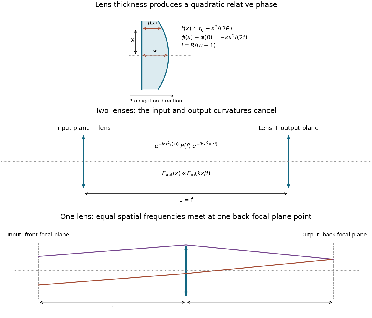

Apply the first lens, propagate, and apply the second lens. Omitting only common prefactors and uniform phases,The coefficients of both and vanish if and only if . The remaining cross term is , soThe Fourier convention here is . Finite clear apertures would truncate the field and limit the spatial-frequency range; the ideal relation assumes the paraxial field fits within both lenses.
Free propagation is convolution with a chirp, . The convolution theorem therefore turns it into multiplication by its Fourier transform. Complete the square:The Gaussian integral then givesThus the wavevector-dependent phase isup to an overall phase convention; after removing the carrier it is . This also follows from .
Normalization qualification: the source keeps a two-dimensional-style prefactor while integrating over only one transverse coordinate. With its literal , there is an additional -independent factor, rather than solely a unit-modulus multiplier. A properly normalized one-dimensional Fresnel propagator has , which cancels the square-root factor above and makes propagation a pure Fourier-domain phase. For example, the literal source kernel multiplies a plane-wave Fourier mode by a factor of magnitude , not one. The spatially dependent phase and the proportional Fourier-transform results remain unchanged. [ref]
Oscillations and Waves by Richard Fitzpatrick. Wave optics, two-dimensional Fourier optics: optical-path expansion and Fourier-domain diffraction
Place the input plane one focal length before a single positive lens and the output plane one focal length after it. The lens maps each incident transverse spatial frequency to its corresponding point in the back focal plane. Referencing the input to the front focal plane removes the otherwise present output phase curvature, giving an exact scaled Fourier transform within the same paraxial model.
A short ray-matrix check makes the geometry explicit. With free propagation and lens matrix ,The vanishing diagonal entries are the Fourier-plane condition; the output is proportional to . The final panel of the original diagram in part a shows the two focal distances. A lens with input immediately on its surface and output at the back focal plane would generally leave a quadratic output phase; the front-focal-plane choice avoids it.
Let , so . The projective measurement has outcome 0 with probability and leaves the state ; outcome 1 has probability and leaves . Alice knows her actual result, so her conditional description is a pure state. Her fidelity of quantum states with the initial state is after outcome 0 or after outcome 1. Its outcome average is .
Bob knows the preparation but not the outcome, so his density matrix is the nonselective postmeasurement stateIt is mixed for and pure only at the endpoints. The relative phase has disappeared because the classical outcome record is unavailable to him.
The undisclosed qubit measurement outcome with an unspecified preparation prior requires care: Charlene has no specified prior over preparations. Consequently the information given does not determine a unique posterior probability for the two outcomes. Under a symmetric ignorance or maximum-entropy prior, her best assignment isMore generally, if her prior mean of is , her assignment is and its fidelity of quantum states with the actual initial state is . Knowing that a measurement occurred guarantees diagonality in its basis, but does not by itself prove . Different descriptions here reflect different available records, rather than different physical outcomes. [ref]
Foundations I: States and Ensembles by John Preskill. Sections 2.3–2.4, density matrices, ensembles and measurement information
Use the common level to subtract the two upper-state energies. The indicated transition satisfiesThe value inherits the rounding of the supplied wavelengths. It is shorter than 397 nm because lies above .
A static electric potential alone cannot confine a charge stably in all three dimensions in a charge-free region. An RF quadrupole ion trap uses a rapidly alternating electric field to provide effective radial confinement; DC endcap fields can supply axial confinement. Near a stable equilibrium, the secular motion sees an approximately harmonic pseudopotential. It has quantized vibrational levels , with separate normal modes along the principal directions. RF Paul trap micromotion is superposed on this slower secular oscillation. For several trapped ions, Coulomb interactions instead give collective normal modes. [ref]
Nobel Lecture: Superposition, entanglement, and raising Schrödinger’s cat by David J. Wineland. Sections III–IV, trapped-ion confinement and quantized motion
The two states are metastable, so a quantum superposition can retain its relative phase much longer than one involving a rapidly decaying state. In the stipulated transition diagram they have no allowed downward electric-dipole transition; real weaker decay channels limit, rather than eliminate, this lifetime advantage. Their distinct energies permit resolved state-selective optical control.
Both levels couple to . Apply coherent beams near 850 nm and 854 nm, detuned from that common intermediate level by a large Rabi detuning . Absorption from one beam and stimulated emission into the other transfer population between the two states without appreciably populating the short-lived intermediate level. Tune the frequency difference to their splitting, including differential AC Stark shifts. In the far-detuned limit,for an initially pure state on two-photon resonance. The controllable relative optical phase sets the rotation axis; the large Rabi detuning suppresses spontaneous-scattering errors. Suitable polarizations and a chosen pair of magnetic sublevels are required in an actual experiment.
Use state-dependent fluorescence. With 397 nm light on and an 866 nm repumper on , an ion initially in is brought into a bright cycling manifold. The repumper prevents population trapping in . An ion in remains dark while the 854 nm light is off, since it has no allowed link to this cycle. A detected bright or dark record therefore measures the qubit in its logical basis by electron shelving.
To reset, apply 854 nm light to empty the shelved state, and use 397 nm plus repumping for Doppler cooling and internal-state preparation. Doppler cooling alone generally does not reach the ground state. In the resolved-sideband and Lamb-Dicke regime, drive the red motional Raman sidebandand then optically repump to with little change in motional occupation. Each cycle removes approximately one vibrational quantum. The state is dark to this red sideband because its matrix element contains . Repeat with appropriate wavevector projections and frequency differences for all modes to be cooled, then optically pump into the selected sublevel. Small recoil during repumping is necessary for a high ground-state probability. [ref]
Nobel Lecture: Superposition, entanglement, and raising Schrödinger’s cat by David J. Wineland. Sections III–IV, fluorescence readout and resolved-sideband control of ion motion
Use the time-ordered network , , . On bits its successive values areThus the network exchanges the two computational-basis states. Since the gates are linear, this basis proof also establishes SWAP gate on arbitrary quantum states.
The Bell states and obeyThe antisymmetric spin singlet state alone has eigenvalue . Its standalone sign is a global phase; a Fredkin gate can make that sign observable relative to the control branch, as in part d.
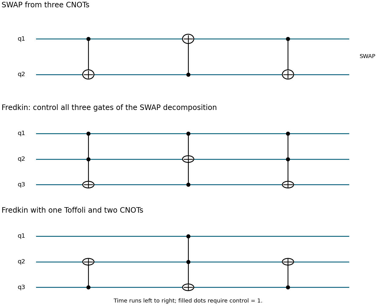
Three controlled-X gates for SWAP, and two decompositions of the Fredkin gate
. Details. 
Control all three CNOTs of the SWAP gate decomposition by qubit 1. This gives, in temporal order,When the first qubit is 0, all three Toffoli gates do nothing. When it is 1, the three lower-wire CNOTs implement SWAP gate. The middle panel of the original diagram shows this controlled network.
Only one Toffoli gate is actually needed. An equivalent circuit isFor input , the first gate forms on wire 2. The second changes wire 3 to , and the final gate gives wire 2 the value . For this is ; for it is . The last panel displays the circuit.
The Hamming-weight obstruction to Fredkin-only Toffoli synthesis means that a network of Fredkin gates alone cannot implement a Toffoli gate on the same three wires: each Fredkin gate preserves computational-basis Hamming weight, whereas Toffoli gate maps to . The same obstruction holds if fixed ancillary bits must be returned unchanged. Conservative classical computation can use extra encoded wires and input-dependent garbage, but that is not an ancilla-free coherent three-qubit Toffoli gate operation. The resources and output encoding would need to be specified before making a different universality claim.
Use basis order , with the ancilla first, and put , . Initially the ancilla is at the north pole of the Bloch sphere. The other two qubits lie on its equator at azimuths , with Bloch vectors .
The four dotted cuts, in left-to-right order, have the explicit normalized vectorsThe first Hadamard gate copies the lower-register amplitudes into two control branches; the Fredkin gate exchanges them only in the second branch; the final Hadamard gate adds and subtracts these branches.
Summing the squared magnitudes of the first four entries of givesMeanwhile , soIdentical input qubits give ; orthogonal equatorial inputs give . The factor one half is an ancilla-interference effect, not a direct projective measurement of the lower qubits individually.
For any joint lower-register state, the probability is , where is its exchange operator. The Bell-state eigenvalues from part a therefore giveFor the spin singlet state, controlled exchange adds a minus sign to the control-1 branch, so the final Hadamard gate puts the ancilla in . For the three symmetric states the ancilla returns to .
The product-state overlap formula cannot be applied to arbitrary entangled lower inputs. All four Bell states have identical one-qubit reduced states , yet the spin singlet state result differs maximally. The network measures exchange symmetry of the joint state, rather than fidelity of quantum states inferred from its two marginals.
Wave plates and polarization phase shifters implement deterministic single-qubit unitaries: a suitable quarter-wave/half-wave/quarter-wave sequence realizes an arbitrary polarization rotation. A deterministic entangling gate on two independently encoded photons needs an effective interaction or additional resources that make one photon's logical action conditional on the other. For example, a sufficiently strong conditional phase followed by Hadamards on the target implements CNOT gate. Ordinary passive linear optics alone does not provide this deterministic interaction on independent polarization qubits. The practical difficulty is that optical nonlinearities at the single-photon level are weak and commonly accompanied by loss or noise; auxiliary photons, measurements and feed-forward trade determinism for resource overhead.
The polarizing beam splitter eigenpolarizations at angle are the orthonormal statesThe first is perfectly transmitted and the second perfectly reflected, from either input port. Port-dependent reflection phases can be fixed by a consistent optical phase convention or compensated locally; they do not alter the transmitted/reflected basis.
Before the gates, write the two Bell states asThe CNOT gate sends the last bit to . Projection onto outcome 0 on qubit 4 therefore requires . After the Hadamard gate on qubit 2, projection onto its outcome 0 contributes for either remaining value of . The unnormalized surviving state isThusThis is entanglement swapping: photons 1 and 3 become entangled even though the joint measurement acts only on their original partners.
For heralded Bell-pair projection with two polarization parity filters, a Hadamard gate followed by computational-basis detection is a measurement in the diagonal polarization basis . It can therefore be realized directly by a polarizing beam splitter at with a photodetector in each output: its transmitted and reflected clicks label and . No separate Hadamard gate plate is required for this measurement.
Conditioning on one photon in each output of the first polarizing beam splitter implements the even -parity filterThe polarizing beam splitter similarly implements the even -parity filter . These are ideal coherent filters, with the optical phases chosen consistently. The all-zero photodetector record projects the upper outputs onto and the lower outputs onto . The two effective bras areTherefore the unnormalized retained state isFor example, the simultaneous Bell contractions require the three pair bits to coincide, leaving only the and terms of the original pair expansion. Each surviving or amplitude is . ConsequentlyThis probability is conditioned on production of all three input pairs, but not yet on successful polarizing beam splitter routing. The routing probability itself is : each nonidentity expectation vanishes on the relevant initial reduced state. Thus, if the question instead regards the routing postselection as already performed,These two denominators describe different conditioning. Neither includes the probability that the three crystals actually emit the required pairs, photodetector inefficiency or undesired multipair events.
A herald tells the experimenter when an entangled resource has actually been prepared while leaving the two resource photons available for subsequent operations. This permits synchronization, conditional storage or switching, and feed-forward. Direct down-conversion emission is probabilistic; inferring that a pair existed by destructively detecting both photons does not leave that same pair available as an input resource.
The second network uses passive optical elements, auxiliary entanglement and detection rather than a strong deterministic photon–photon CNOT gate interaction. Its smaller success rate can be acceptable if trials are inexpensive and successful events are reliably announced. Heralding is still probabilistic, not deterministic on demand; losses, dark counts and multiple-pair emission can give false or degraded heralds. The ideal result assumes the specified input pairs and valid detection model, so it should not be confused with a complete laboratory production efficiency.
Use , , and . Only one interaction term acts on each of the two quantum states. HenceThe interaction exchanges one atomic excitation with one field quantum. The square-root factor is the photon-number enhancement of the transition matrix element.
The total excitation operator commutes with the Hamiltonian. Each sector with is therefore spanned by , and no term connects it to a sector of different excitation number.
In that ordered basis, with the source's Rabi detuning ,The first term is the common sector energy; the remaining diagonal entries record the bare Rabi detuning and the off-diagonal terms exchange the excitation.
The isolated ground sector of the Jaynes-Cummings model is an important exception to a statement that the entire Hilbert space consists of such pairs: has no partner and is annihilated by both interaction terms. It is a one-dimensional invariant sector with energy . The full decomposition is this one-dimensional sector plus all the two-dimensional sectors above.
Subtract the common sector energy and call the remaining eigenvalue . Its characteristic equation isThe dressed-state energies are consequentlyOn resonance their splitting is ; far off resonance the eigenstates approach the uncoupled quantum states with small dispersive energy shifts. The eigenvalue splitting is an angular-frequency difference , so an ordinary frequency would be .
The requested bare labels require . Their four energies areAmong these four, the pair that is fully present in one interacting sector is . Its center is and its dressed branches areTheir endpoint values at and are the same, . At they are . The avoided crossing therefore has resonant gapAt the three horizontal-axis landmarks, the bare energies divided by are respectivelywhich specifies the vertical-axis labeling without assigning an unstated numerical . The original plot below uses illustrative and and shows this complete central doublet together with all four bare lines.
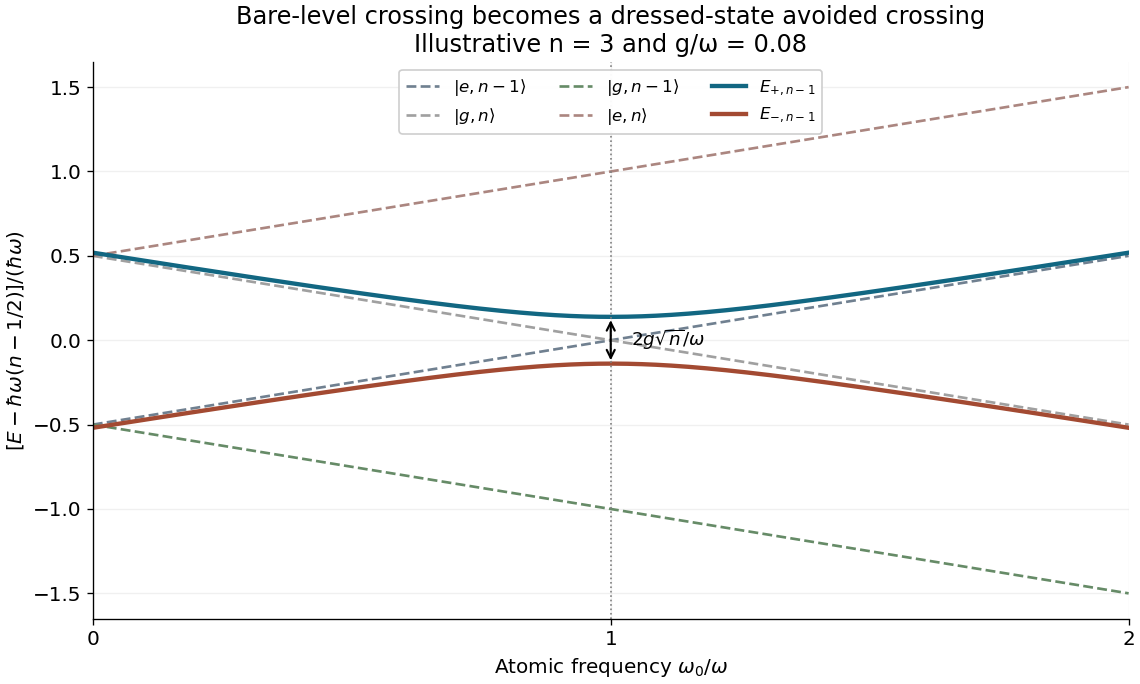
Four bare levels and the complete dressed doublet contained among them in the Jaynes-Cummings model
. Details. 
Sector qualification: the outer displayed state couples to , outside the requested bare set. Likewise couples to if ; for it is the isolated . Thus the four-state set cannot be diagonalized as a closed four-dimensional block. If branches associated with these outer states are also desired, complete those neighboring sectors and use the formula in part c with indices and .
Finally, “adjacent dressed states” within the shown resonant pair have the gap just boxed. Adjacent rungs of the dressed ladder are not equally spaced: at resonance,When neighboring doublets remain ordered, the gap between their nearest branches is . This distinguishes the within-doublet Rabi splitting from differences between adjacent excitation sectors.
Articles by others on the same topic
There are currently no matching articles.