Past exam of the mathematical and Computational Biology course of the University of Cambridge / 2024 / Paper 2 / B4

Write

m_{i} \in {0, 1}

for the true DNA methylation status and

o_{i}

for its observation. The observation likelihood function is a binary symmetric channel, so

lo g p (o ∣ m) = \sum_{i = 0}^{99} {lo g (0.8), lo g (0.2), o_{i} = m_{i}, o_{i} \neq = m_{i} .

(1)

For the loop suggested in the practical, set

p_{i} = (0.1, 0.5, 0.9)_{m_{i - 1} + m_{i + 1}}

and add

lo g p_{i}

when

m_{i} = 1

, or

lo g (1 - p_{i})

otherwise. The following independent implementation combines these terms without multiplying many small numbers:

import numpy as np

def methylation_score(pattern, observed):
    """Conditional-product score used by the practical's natural loop filling."""
    pattern=np.asarray(pattern,dtype=int);observed=np.asarray(observed,dtype=int)
    if pattern[0]!=1 or pattern[-1]!=1:return -np.inf
    neighbour_sum=pattern[:-2]+pattern[2:]
    p=np.array([.1,.5,.9])[neighbour_sum]
    prior_terms=np.where(pattern[1:-1]==1,p,1-p)
    observation_terms=np.where(pattern==observed,.8,.2)
    return float(np.log(prior_terms).sum()+np.log(observation_terms).sum())

log_likelihood = methylation_score
print(f"{log_likelihood(obs, obs):.2f}")

The conditional-product log score at the observed pattern is $- 102.14$ . The endpoint observations are included once each, while the endpoint statuses are fixed rather than assigned an additional prior probability.

There is a modeling qualification: multiplying the specified neighbour conditional probabilities gives a pseudolikelihood, not generally the joint probability distribution having those conditional probabilities. Thus the function above defines the practical's conditional-product target; the pure observation log-likelihood at

m = o

would instead be

100 lo g (0.8) = - 22.3144

If the neighbour probabilities are intended literally as full conditionals of a Markov random field, a coherent alternative has edge weights

T_{aa} = 3/4

and

T_{ab} = 1/4

for

a \neq = b

, with both endpoints fixed. Given two equal neighbours, the matching centre has conditional odds

(3/4)^{2} : (1/4)^{2} = 9 : 1

; mixed neighbours give equal weights. Consequently its unnormalized posterior probability has log score

ℓ_{J} (m; o) = \sum_{i = 0}^{98} lo g T_{m_{i} m_{i + 1}} + lo g p (o ∣ m) .

(2)

For this alternative,

ℓ_{J} (o; o) = - 94.7394

before the constant associated with conditioning the endpoints. It can be implemented as follows, but its numerical results must not be mixed with the conditional-product results in the remaining parts:

def joint_methylation_score(pattern,observed):
    """Coherent nearest-neighbour model with the specified full conditionals."""
    pattern=np.asarray(pattern,dtype=int);observed=np.asarray(observed,dtype=int)
    if pattern[0]!=1 or pattern[-1]!=1:return -np.inf
    edges=np.where(pattern[1:]==pattern[:-1],.75,.25)
    emissions=np.where(pattern==observed,.8,.2)
    return float(np.log(edges).sum()+np.log(emissions).sum())

b

 0  0

Solution

 0  0

A single randomly chosen internal-site flip is a symmetric proposal: the reverse flip has the same probability

1/98

. Therefore the Metropolis–Hastings algorithm accepts with

α = min {1, exp (s (m^{'}; o) - s (m; o))} .

(1)

Comparing logarithms avoids overflow. On rejection the old state must be retained, including a repeated copy in the stored Markov chain; retaining only accepted states would sample a different distribution. This implementation also stores the actual initial state at row zero:

def sample_methylation(observed, nsteps=5000, seed=2024, score=methylation_score):
    rng=np.random.default_rng(seed)
    state=rng.integers(0,2,size=len(observed));state[[0,-1]]=1
    states=np.empty((nsteps,len(state)),dtype=int);values=np.empty(nsteps)
    states[0]=state;values[0]=score(state,observed)
    accepted=0
    for t in range(1,nsteps):
        candidate=state.copy();site=rng.integers(1,len(state)-1)
        candidate[site]=1-candidate[site]
        trial=score(candidate,observed)
        if np.log(rng.random())<min(0.,trial-values[t-1]):
            state=candidate;values[t]=trial;accepted+=1
        else:values[t]=values[t-1]
        states[t]=state
    return values,states,accepted/(nsteps-1)

lls, meths, acceptance = sample_methylation(obs, nsteps=5000, seed=2024)
import matplotlib.pyplot as plt
plt.plot(lls)
plt.xlabel("Stored state index")
plt.ylabel("Conditional-product log score")
plt.show()

For this random-number convention, the acceptance fraction is approximately $0.157$ . The trace climbs substantially during its first several thousand updates, so a small fixed burn-in such as 100 iterations would discard too little of the initial transient. Five thousand single-site proposals are only about fifty updates per site on average.

Figure 1.

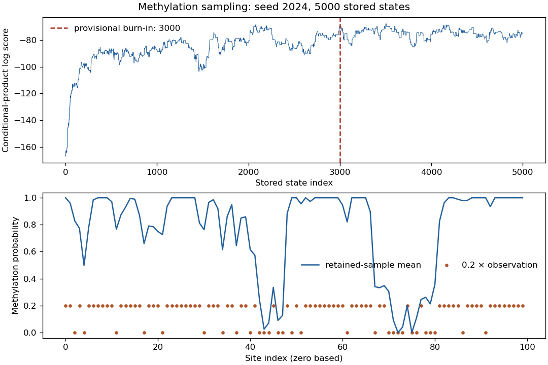
Conditional-product sampling trace and retained-sample methylation profile, with a provisional burn-in of 3000 stored states

. Details.

c

 0  0

Solution

 0  0

For a binary state, its expected value is its probability of being one. Hence the Monte Carlo method estimate of the posterior methylation profile under the chosen target is

p_{i} = \frac{1}{N - B} \sum_{t = B}^{N - 1} m_{i}^{(t)} .

(1)

The averaging axis must be zero: average over sampled patterns while keeping the site index. A provisional choice for this particular trace is $B = 3000$ , retaining 2000 states:

def mean_methylation(meths, burnin):
    if not 0 <= burnin < len(meths):
        raise ValueError("burn-in must leave at least one state")
    return np.asarray(meths)[burnin:].mean(axis=0)

burnin = 3000
profile_estimate = mean_methylation(meths, burnin)
print(lls[burnin:].mean())
plt.plot(profile_estimate, label="retained-sample mean")
plt.scatter(np.arange(len(obs)), .2*obs, s=10, label="0.2 × observation")
plt.xlabel("Site index")
plt.ylabel("Methylation probability")
plt.legend()
plt.show()

The retained mean log score is $- 74.8895$ , and the profile is shown below the trace in part (b). The fixed endpoints have estimate exactly one; adjacent sites are often smoothed into methylated or unmethylated stretches despite individual conflicting observations. The rescaled observations are only a visual comparison and are not another estimate of the posterior probability.

This is a finite-chain estimate for the conditional-product target defined in part (a). A burn-in chosen by inspection does not establish convergence, and the long excursions in this short Markov chain leave substantial uncertainty in individual-site estimates; several longer runs would be needed for precise inference. To sample the coherent joint alternative instead, pass score=joint_methylation_score and inspect that new trace before choosing its own burn-in.

d

 0  0

Solution

 0  0

The retained mean conditional-product log score, $- 74.89$ , is higher than the observed-pattern score, $- 102.14$ , because sampled patterns can improve agreement between neighbouring CpG sites while tolerating some observational errors. The observation-matching pattern maximizes the observation likelihood function alone, whereas this score also rewards the assumed spatial structure, and its posterior mean is not its maximum.

Past exam of the mathematical and Computational Biology course of the University of Cambridge / 2024 / Paper 2 / B4

a

Solution

b

Solution

c

Solution

d

Solution

 Ancestors (11)

 Discussion (0)

 Articles by others on the same topic (0)

Past exam of the mathematical and Computational Biology course of the University of Cambridge / 2024 / Paper 2 / B4

 Discussion (0)  Subscribe (1)

 Discussion (0)