Represent the leading real pattern by . Before forcing, continuous translation symmetry acts as , and spatial reflection acts as . Equivariance excludes quadratic terms and permits a linear term and at cubic order. Symmetry under reflection makes their coefficients real. A supercritical bifurcation has a saturating cubic coefficient; rescaling amplitude and time makes it . The imperfection has a Fourier component at the same wavenumber, so its resonant projection contributes an additive real coefficient. On the spatially uniform wave envelope subspace the amplitude equation is therefore . Allowing modulations would additionally produce the spatial terms of the real Ginzburg–Landau equation.
For a forcing pattern moving in the positive direction, its laboratory-frame coefficient is , where is proportional to after converting to slow time. The comoving amplitude is , since the fast carrier becomes . Differentiation givesA constant phase choice makes , and complex conjugation reverses the sign of , so take . Put and . The rescaled linear coefficients are and , and the forcing becomes one. Below the rescaled variables are renamed , giving the directly forced cubic amplitude equation.
Write . A steady complex amplitude obeys , soThus every positive intensity root gives exactly one steady phase, and is impossible. The cubic intensity polynomial is . Its positive steady branch can be parameterized completely asThe two formulae join smoothly as a single curve at the maximum radius ; this joining point is not a saddle-node bifurcation. A turning point with respect to satisfies . Subtracting the equilibrium and derivative conditions givesThese points lie on . Since , its maximum is . Therefore there is exactly one distinct steady state for every when . One can also see uniqueness directly: is increasing and is decreasing when no turning points exist, and their respective ranges meet only at their common endpoint. At the equality there is a cusp bifurcation with a triple intensity root at .
When , the two turning intensities satisfy . Define and ; the curve has a local minimum at the former and a local maximum at the latter, with . There are three distinct steady intensities for , two distinct ones at an endpoint, and one otherwise. The bifurcation diagrams below show the folded small- curves and the unfurled large- curve, together with the linear stability calculated next. Both ends of the full branch have as , while its middle reaches the finite maximum .
Let the equilibrium be and write . The linearization of the cubic term gives . Therefore the real stability matrix isIts eigenvalues obeyThe square root may be imaginary; stability uses real parts. The determinant is exactly , so a zero eigenvalue occurs only at the turning points derived above. Away from the cusp those are ordinary saddle-node bifurcations; the parameterization joining point has .
At a candidate Hopf bifurcation, the trace vanishes: . Substitution into the steady cubic gives , which has one positive root. The pair is genuinely imaginary only ifThus and, equivalently,This direct calculation proves the threshold without needing the additional monotonicity assumption. The equality gives a double-zero eigenvalue, not an ordinary Hopf bifurcation. Along a fixed- branch, implicit differentiation gives ; at this crossing . A nonzero nonlinear Hopf coefficient then gives the usual Hopf bifurcation.
The fold and Hopf thresholds of a directly forced cubic amplitude divide the diagrams into three regimes. At noncritical points the two eigenvalues, counted with multiplicity by the signs of their real parts, are classified as follows:
- For , there is one equilibrium for every . It has two stable eigenvalues for and two unstable eigenvalues for .
- For , the largest-amplitude branch has two stable eigenvalues; the intermediate-amplitude branch has one stable and one unstable eigenvalue. The smallest-amplitude branch emerging from the lower fold has two stable eigenvalues up to its Hopf crossing, and two unstable eigenvalues beyond it. The relative location of the Hopf point and the other fold in is not fixed throughout this interval.
- For , the largest-amplitude branch again has two stable eigenvalues, the intermediate branch has one of each, and the smallest-amplitude branch has two unstable eigenvalues. The trace-zero point lies on the saddle segment and is not a Hopf bifurcation because its determinant is negative.
At a fold one eigenvalue is zero; at a Hopf point the pair has zero real part. These nonhyperbolic points are marked separately in the sketches.
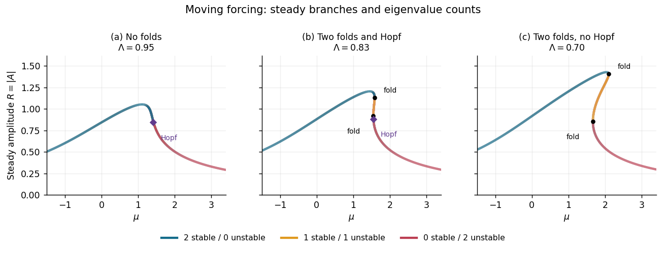
Steady amplitudes of the moving forced pattern, with folds, Hopf points and stable/unstable eigenvalue counts in all three regimes
. Details. 
Articles by others on the same topic
There are currently no matching articles.