Past exam of the mathematics course of the University of Cambridge / 2004 / ia / Paper 2 / 7B (Differential Equations)

Introduce the velocity variable $v=\dot{x}$. The second-order differential equation becomes the autonomous planar systemA critical point of a dynamical system is a point where both components of the vector field vanish: here $v=0$ and $f(x,0)=0$. It is a stationary solution in the phase plane. The Jacobian matrix at each such point gives the local linear stability of a planar equilibrium. For the equations below, a conserved energy also determines the nonlinear phase portrait; this is important because purely imaginary eigenvalues alone do not generally prove that an equilibrium is a center equilibrium.

Here the autonomous planar system is $\dot{x}=v$, $\dot{v}=-\cos x$. Its equilibrium points areThe Jacobian matrix isFor even $n$, the eigenvalues are $1,-1$, so these points are unstable saddle equilibria. Writing $\xi =x-x_{\ast }$, their local unstable and stable directions are $v=\xi$ and $v=-\xi$ respectively. For odd $n$, the eigenvalues are $i,-i$.

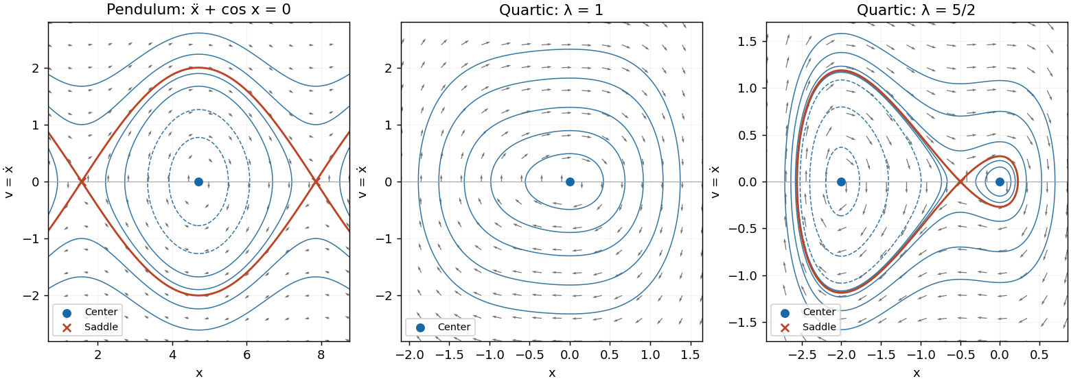
To classify the latter points nonlinearly, differentiate the first integralAt $x_{\ast }=3\pi /2+2m\pi$ this energy has a strict local minimum. Its nearby level sets are closed curves, proving that the odd-$n$ points are stable center equilibria, with no attraction to the center. The phase portrait consists of closed oscillatory orbits for $-1<H<1$, heteroclinic orbits at $H=1$ joining consecutive saddle equilibria, and open rotating orbits for $H>1$. The separating curves haveAbove the horizontal axis $\dot{x}=v>0$, so flow is rightward; below it flow is leftward. The closed orbits are clockwise, and these same signs orient every separating and rotating orbit.

For both parameters the autonomous planar system is $\dot{x}=v$, $\dot{v}=-x(x^2+\lambda x+1)$. It has the conserved energyIndeed $\dot{H}=v\dot{v}+V_{\lambda }^{\prime }(x)\dot{x}=0$. At any equilibrium point $(x_{\ast },0)$ the eigenvalues satisfy

For $\lambda =1$, the quadratic $x^2+x+1$ is strictly positive, so the only equilibrium point is $(0,0)$, with eigenvalues $\pm i$. Since $V_1^{\prime }(x)$ has the sign of $x$, $V_1$ has a unique strict minimum at zero and tends to infinity in both directions. All positive energy levels are closed curves surrounding this stable center equilibrium. They are clockwise: rightward when $v>0$ and leftward when $v<0$.

For $\lambda =5/2$, factor $x^2+(5/2)x+1=(x+2)(x+1/2)$. The three equilibrium points and their classifications areThe two center equilibria are stable but not asymptotically stable; the saddle equilibrium is unstable. At the saddle equilibrium the local unstable and stable directions are $v=(\sqrt{3}/2)(x+1/2)$ and $v=-(\sqrt{3}/2)(x+1/2)$.

The potential values are $V(-2)=-2/3$, $V(0)=0$, and $V(-1/2)=7/192$. Consequently there are closed loops around the left center for $-2/3<H<0$, closed loops in both wells for $0<H<7/192$, and a figure-eight pair of homoclinic orbits at $H=7/192$. At $H=0$ the right center is a stationary point while the left well still has a closed orbit. For $H>7/192$, each closed curve encircles both centers and the saddle.

The two homoclinic orbits satisfy $v=\pm \sqrt{2(7/192-V(x))}$. Their outer turning points can be located exactly fromEvery nonstationary energy curve is oriented to the right in the upper half-plane and to the left in the lower half-plane. The sketches show the closed curves, the separating orbits, the stable and unstable saddle directions and the direction of flow.