The origin is an ordinary point, since the coefficients of the second-order linear differential equation are polynomials. Seek a power series . Matching the coefficients of and gives . Matching the coefficient of givesThus the four residue classes of indices modulo four evolve separately. The initial conditions for the first solution give , , and henceThe second set of initial conditions gives , , andAn empty product equals one. In either power series, the ratio of successive nonzero terms tends to zero for every fixed : the coefficient ratio is of order , while the power increases by four. The ratio test therefore proves convergence for every , and termwise differentiation verifies the differential equation. These normalized solutions are linearly independent.
For their Wronskian , differentiating and substituting the differential equation givesThus the Abel identity yieldsOn the interval containing zero where has no zero,Since , integration proves the requested reduction of order formula:This is a local formula around the origin, as requested. The power series define both solutions globally; an ordinary integral through a zero of is not intended. Reduction of order across a zero of the known solution instead uses continuation of the actual solution.
Substitute the linear recurrence relation for each of and in the discrete Wronskian:Iterating givesNo division was used, so vanishing cause no exception.
For constant coefficients, seek a solution . The characteristic equation of a linear recurrence is . Choose with . Its roots are and , since . For the two resulting solutions,It is independent of , exactly as the product identity predicts when .
When the roots are distinct and the discrete Wronskian is nonzero. At or , the two displayed solutions coincide and ; the identity still holds. If an independent pair is wanted at these endpoints, take and , where or respectively. Direct substitution verifies both, and their discrete Wronskian is .
Introduce the velocity variable . The second-order differential equation becomes the autonomous planar systemA critical point of a dynamical system is a point where both components of the vector field vanish: here and . It is a stationary solution in the phase plane. The Jacobian matrix at each such point gives the local linear stability of a planar equilibrium. For the equations below, a conserved energy also determines the nonlinear phase portrait; this is important because purely imaginary eigenvalues alone do not generally prove that an equilibrium is a center equilibrium.
Here the autonomous planar system is , . Its equilibrium points areThe Jacobian matrix isFor even , the eigenvalues are , so these points are unstable saddle equilibria. Writing , their local unstable and stable directions are and respectively. For odd , the eigenvalues are .
To classify the latter points nonlinearly, differentiate the first integralAt this energy has a strict local minimum. Its nearby level sets are closed curves, proving that the odd- points are stable center equilibria, with no attraction to the center. The phase portrait consists of closed oscillatory orbits for , heteroclinic orbits at joining consecutive saddle equilibria, and open rotating orbits for . The separating curves haveAbove the horizontal axis , so flow is rightward; below it flow is leftward. The closed orbits are clockwise, and these same signs orient every separating and rotating orbit.
For both parameters the autonomous planar system is , . It has the conserved energyIndeed . At any equilibrium point the eigenvalues satisfy
For , the quadratic is strictly positive, so the only equilibrium point is , with eigenvalues . Since has the sign of , has a unique strict minimum at zero and tends to infinity in both directions. All positive energy levels are closed curves surrounding this stable center equilibrium. They are clockwise: rightward when and leftward when .
For , factor . The three equilibrium points and their classifications areThe two center equilibria are stable but not asymptotically stable; the saddle equilibrium is unstable. At the saddle equilibrium the local unstable and stable directions are and .
The potential values are , , and . Consequently there are closed loops around the left center for , closed loops in both wells for , and a figure-eight pair of homoclinic orbits at . At the right center is a stationary point while the left well still has a closed orbit. For , each closed curve encircles both centers and the saddle.
The two homoclinic orbits satisfy . Their outer turning points can be located exactly fromEvery nonstationary energy curve is oriented to the right in the upper half-plane and to the left in the lower half-plane. The sketches show the closed curves, the separating orbits, the stable and unstable saddle directions and the direction of flow.
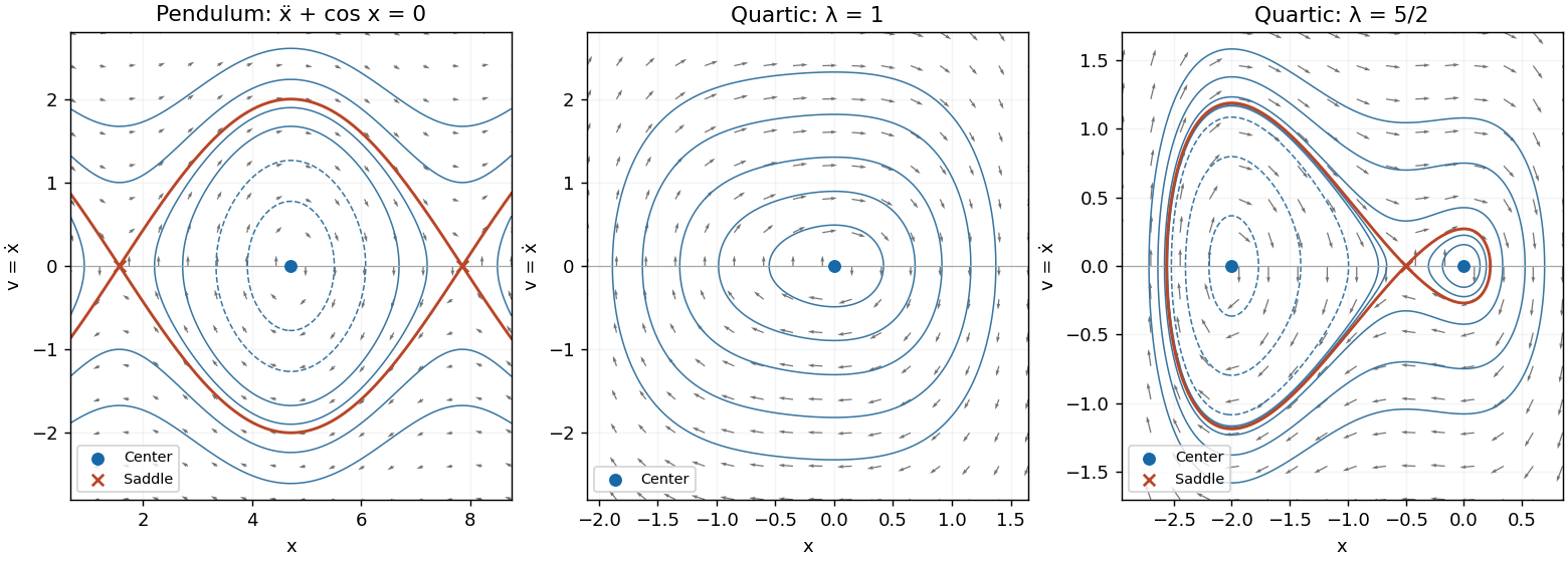
Clockwise phase flows, alternating pendulum saddles and centers, and the one-well and two-well quartic potentials
. Details. 
Write the linear differential equation as , withIts characteristic polynomial is . Thus a choice of eigenvalues and eigenvectors isThe distinct eigenvalues give two linearly independent solutions, and the general complex solution isReal solutions have . Equivalently,They spiral counterclockwise towards the origin, which is a stable spiral.
In a forced linear differential equation, resonance in a differential equation occurs when exponential forcing excites a mode with the same exponent as its eigenvalue, producing a polynomial factor such as multiplying that exponential. Merely matching an exponent is not enough: its projection onto that mode must be nonzero. Here still decays in absolute magnitude because the real part of is negative; resonance refers to this extra factor, not necessarily to unbounded growth.
For each forcing vector, resolve it in the eigenvector basis:If is the coefficient of the th eigenvector, its scalar equation is . Multiplying by and integrating shows that the contribution is , whereas a contribution is . Therefore the exact conditions for no resonant response areUnder these conditions one particular solution iswhich contains no factor of . For a real forcing, and , and the two boxed conditions are conjugate to each other.
The probability generating function isFor independent random variables, the bounded factors and have factorizing expectation, soThis includes complex in the indicated disk by absolute convergence.
For the dice construction, encode the labels of an ordinary die by . Its probability generating function is . A useful factorization into polynomial factors isUse redistribution of polynomial factors for dice to defineBoth polynomials have nonnegative integer coefficients, no constant term, and coefficient sum six. They therefore describe fair six-sided dice with strictly positive face labelsWhen these dice are thrown with independent outcomes, the sum has probability generating function . Equality of coefficients proves equality of every sum probability, including all totals from two to twelve, with zero probability outside that range. Both dice are nonstandard, completing the construction.
For events with , the conditional probability isUse the sample space , where the first coordinate is the chosen coin and the other coordinates record which of its two physically distinguished faces lands upwards on each toss. There are equally likely elementary outcomes. Label the double-headed coin by one. For that coin both face indices mean heads; for each other coin only face index one means heads. In particular, strings of observed heads and tails are not equally likely outcomes.
Let be the event that the first three tosses show heads. With coin one all sixteen face-index strings are permitted. For each ordinary coin the first three indices must be one and the fourth is free, giving two strings. Thus . Of these outcomes, sixteen from the double-headed coin and one from each ordinary coin also have a fourth head. HenceEquivalently, Bayes' theorem gives conditional probability of having selected the double-headed coin after ; the fourth-head probability is then . The tosses are independent conditional on the selected coin, while mixing over the same coin explains their unconditional dependence.
Take as the rate of the exponential distribution. By independence, the joint probability density of the original pair is on . Put , . The inverse change of variables isIts Jacobian determinant isUsing the absolute value in the change of variables formula, the transformed joint probability density isand zero otherwise. The support is the entire positive quadrant, and the factors are separately normalized:Integrating out either variable therefore yields these factors as the marginal densities. Factorization of the joint probability density proves independence, withThe sum has a shape-two gamma distribution, and the ratio has a beta-prime distribution with parameters one and one, independent of . Its cumulative distribution function is for .
Because the events are pairwise disjoint events, their count can only be zero or one. The event that the count is zero is the complement of an event of their union. Finite additivity therefore gives
Now use for the fixed number of independently located ships. Normalize the radius to one and write their positions as unit vectors . A point on the sphere is reached by ship precisely when , so each ship reaches an open hemisphere. Coverage fails exactly when there is a unit vector with for every . Equivalently, all ship positions lie in some closed hemisphere.
With probability one no pair of ship vectors is antipodal and no three are linearly dependent: the exceptional choices lie on sets of zero surface area. For such a configuration, containment in a closed hemisphere implies containment in an open hemisphere. To see this, choose its inward normal , so . At most two vectors lie on its boundary. If there are two, their sum has positive dot product with each, since they are not antipodal; if there is one, use that vector itself. Perturb slightly in this direction. The boundary dot products become positive while all already positive dot products remain positive. Thus the strict and non-strict containment conditions have the same probability here.
Condition on the unoriented axes . Choose representatives by any fixed sign convention. By uniform sampling and independence, the actual positions are with independent fair signs . Conditional on these axes, each of the sign choices has probability .
The great circles partition the sphere into open regions. In each region the sign vector is constant. No sign vector labels two different regions: its strict inequalities define a convex cone, and normalized line segments within that cone connect any two points of its spherical section. The regions of a general-position great-circle arrangement therefore yield exactly realized sign vectors.
The chosen positions lie in an open hemisphere if and only if some has for every , that is, for every . Failure of coverage thus corresponds exactly to one of the realized sign choices. These choices are mutually exclusive events, each of conditional probability , so the first part applies:The result is independent of the axes. Averaging gives the coverage of a sphere by random open hemispheres:For this is zero; for it is . If no ship lands, coverage has probability zero separately. The counting uses equiprobable orientation signs, not an assumption that the spherical regions have equal area.
Articles by others on the same topic
There are currently no matching articles.