Past exam of the mathematics course of the University of Cambridge / 2004 / iii / Paper 70 / 3

Let the original abscissae be $x_i=ih$ and vary only the ordinate of vertex $i$. Under Chaikin subdivision, the two child values on an edge are $\frac{3}{4}{y}_j+\frac{1}{4}{y}_{j+1}$ and $\frac{1}{4}{y}_j+\frac{3}{4}{y}_{j+1}$. All influence weights are nonnegative, so no cancellation removes an active descendant.

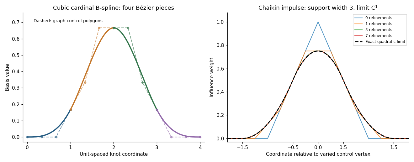
At level $r$ the spacing is $h_r=h/2^r$. If the leftmost influenced vertex is at $a_r$, the next leftmost is the quarter point on the preceding edge, $a_{r+1}=a_r-3h_r/4$; the rightmost advances by the same amount. Starting at $x_i$, the influenced vertex range is thereforeThe neighboring zero vertices bound any extra affected polygon segments by one refined spacing, which tends to zero. Passing to the limit givesIt spans three original grid intervals, with its endpoints at original edge centers. Positive descendant weights occur arbitrarily close to each endpoint, so this is the exact support closure. The support of a stationary subdivision scheme concerns the limit curve, not only the first pair of adjacent original edges. This describes interior vertices or an infinite uniform sequence; a finite open polygon needs an endpoint convention.

Use coordinates in which the current spacing is $h$. On the first child subgrid, the polynomial candidate ison the second it isFor arbitrary sufficiently long uniformly spaced data, all refined vertices can lie on one degree-$n$ polynomial only if these two candidate polynomials agree. They agree with $P$ when $n=0,1$. For $P(x)=a{x}^2+bx+c$, expansion givesThus quadratics preserve their degree, although not the same values.

For a polynomial of degree $n\ge 3$, subtract the two finite Taylor expansions. The first-derivative term cancels, while the leading nonzero differential term isIf the leading coefficient of $P$ is $a_n\ne 0$, this difference has nonzero coefficient $a_{n}n(n-1)(n-2)h^3/32$ at degree $n-3$; the higher derivatives have lower degree and cannot cancel it. Therefore the polynomial degree preservation under Chaikin subdivision holds exactly forThis is a general refinement property, independent of accidental interpolation through a small finite number of vertices.

Use the influence result and quadratic degree preservation to find each local limit piece, rather than assuming its smoothness. On $[x_i-h/2,x_i+h/2]$, only $y_{i-1},y_i,y_{i+1}$ matter. Extend these three values to a quadratic $P(x)=a{x}^2+bx+c$ across the uniform grid. Every refinement adds $3a{h}_r^2/16$, so the accumulated offset tends toBy locality this gives the same limit as the original data on the chosen interval. Put $t=(x-x_i)/h$ and $D_i=y_{i-1}-2y_i+y_{i+1}$. The limit piece is consequentlyAt the right edge center it hasThe next piece gives the same value and derivative at its left endpoint. The second derivatives on the two sides are instead $D_i/h^2$ and $D_{i+1}/h^2$, which generally differ. HenceThere is one continuous derivative in addition to the continuous curve itself. Special data such as a globally quadratic sequence can make higher derivatives match.

The rule is linear in the ordinates and translation invariant on the uniform grid, so write $s(x)={\sum }_i{y}_i\beta ((x-x_i)/h)$. Find its Chaikin basis function by setting $y_0=1$ and every other ordinate to zero. The central local piece just derived has $D_0=-2$ and gives $\beta (t)=3/4-t^2$ for $|t|\le 1/2$. On the next interval, the interpolating quadratic through values $1,0,0$ at abscissae $0,1,2$ is $\frac{1}{2}(t-1)(t-2)$. Adding its limiting offset $1/8$ gives $\frac{1}{2}(3/2-t{)}^2$. Reflection gives the left interval, and locality gives zero outside. ThusThis is a centered quadratic cardinal B-spline. It is nonnegative, and its integer translates form a partition of unity because refinement preserves constant data. Its support has width three, and its first derivative agrees at the half-integer knots while its second generally jumps, consistent with the earlier calculations.