Use vectors in three-dimensional Euclidean space, with the usual dot product and cross product. The following explicit assignments compute the circumcenter of a tetrahedron:General position means . The reciprocal cross-product identities give , and . Consequentlyand likewise for . Thus is the unique point equidistant from the four vertices. It can lie outside the tetrahedron; no inside constraint should be imposed.
Compute twice the four opposite face areas and their weighted vertex average:These positive weights make an interior convex combination. To verify the incenter of a tetrahedron, put . The altitude from to its opposite face is . Signed distance to that face is affine and vanishes at the other three vertices, so has distance . The same argument works for every face. HenceThe sphere of radius centered at is tangent to all four faces. Equality of the four distances conversely forces these face-area weights, proving uniqueness.
The degree- Bernstein basis on isThe associated Bézier curve is . The basis is nonnegative and has partition of unity, since . Thus the curve is a convex combination of its control points, giving the convex hull enclosure useful for geometric bounds. The same identity makes the construction invariant under application of affine functions.
It interpolates its endpoint controls, , , and its endpoint tangent vectors are and . These follow fromThe control polygon therefore gives direct geometric editing and tangent control. Repeated interpolation by the De Casteljau algorithm evaluates and subdivides the curve without converting to a monomial representation. Together, positive geometric weights, simple endpoint behavior and stable subdivision make this basis useful in computer aided geometric design.
A degree- B-spline basis keeps the positive partition of unity and convex hull properties while introducing local support. At a generic parameter value, only consecutive basis functions are nonzero. Moving one control point therefore changes only its support interval, unlike a generic interior Bézier curve control, which affects the whole polynomial segment.
Many low-degree pieces can represent a long curve with automatic continuity. At a knot of multiplicity , the generic continuity is ; simple cubic knots give . Knot positions and multiplicities control the placement of detail and joins. Knot insertion can refine the representation without changing the curve, and local refinement avoids raising the global polynomial degree. Thus B-splines combine geometric bounds, local editing and controlled smoothness with a fixed low degree. Clamped end knots can also give endpoint interpolation.
Scale the equal intervals to unit length. A nonzero compactly supported cubic B-spline with maximum continuity is , so its fourth derivative is a sum of impulses at the knots. Equivalently it is a combination of truncated cubes,To vanish to the right of its support, the polynomial tail must be identically zero. Expanding that tail requires for . Four or fewer distinct knots give a full-rank Vandermonde matrix and only the zero solution. Hence a nonzero function requires at least five knots, or four intervals. At knots , the one-dimensional nullspace has coefficients proportional to . The unscaled combination integrates to six on , so unit-integral cardinal normalization gives:This is the Cardinal cubic B-spline, nonnegative with support . To obtain its cubic B-spline Bézier extraction, use local parameter on interval . The four power-form numerators, with a common divisor six, areFor , the cubic Bernstein basis coefficients are , , , . Applying this conversion givesEach scalar row describes a cubic Bézier curve graph piece with abscissa controls . The truncated-cube construction proves value, first- and second-derivative agreement at all joins, including the zero exterior. Minimum support and maximum continuity determine the basis up to a scalar; the displayed normalization fixes that remaining freedom.
Let the original abscissae be and vary only the ordinate of vertex . Under Chaikin subdivision, the two child values on an edge are and . All influence weights are nonnegative, so no cancellation removes an active descendant.
At level the spacing is . If the leftmost influenced vertex is at , the next leftmost is the quarter point on the preceding edge, ; the rightmost advances by the same amount. Starting at , the influenced vertex range is thereforeThe neighboring zero vertices bound any extra affected polygon segments by one refined spacing, which tends to zero. Passing to the limit givesIt spans three original grid intervals, with its endpoints at original edge centers. Positive descendant weights occur arbitrarily close to each endpoint, so this is the exact support closure. The support of a stationary subdivision scheme concerns the limit curve, not only the first pair of adjacent original edges. This describes interior vertices or an infinite uniform sequence; a finite open polygon needs an endpoint convention.
Use coordinates in which the current spacing is . On the first child subgrid, the polynomial candidate ison the second it isFor arbitrary sufficiently long uniformly spaced data, all refined vertices can lie on one degree- polynomial only if these two candidate polynomials agree. They agree with when . For , expansion givesThus quadratics preserve their degree, although not the same values.
For a polynomial of degree , subtract the two finite Taylor expansions. The first-derivative term cancels, while the leading nonzero differential term isIf the leading coefficient of is , this difference has nonzero coefficient at degree ; the higher derivatives have lower degree and cannot cancel it. Therefore the polynomial degree preservation under Chaikin subdivision holds exactly forThis is a general refinement property, independent of accidental interpolation through a small finite number of vertices.
Use the influence result and quadratic degree preservation to find each local limit piece, rather than assuming its smoothness. On , only matter. Extend these three values to a quadratic across the uniform grid. Every refinement adds , so the accumulated offset tends toBy locality this gives the same limit as the original data on the chosen interval. Put and . The limit piece is consequentlyAt the right edge center it hasThe next piece gives the same value and derivative at its left endpoint. The second derivatives on the two sides are instead and , which generally differ. HenceThere is one continuous derivative in addition to the continuous curve itself. Special data such as a globally quadratic sequence can make higher derivatives match.
The rule is linear in the ordinates and translation invariant on the uniform grid, so write . Find its Chaikin basis function by setting and every other ordinate to zero. The central local piece just derived has and gives for . On the next interval, the interpolating quadratic through values at abscissae is . Adding its limiting offset gives . Reflection gives the left interval, and locality gives zero outside. ThusThis is a centered quadratic cardinal B-spline. It is nonnegative, and its integer translates form a partition of unity because refinement preserves constant data. Its support has width three, and its first derivative agrees at the half-integer knots while its second generally jumps, consistent with the earlier calculations.
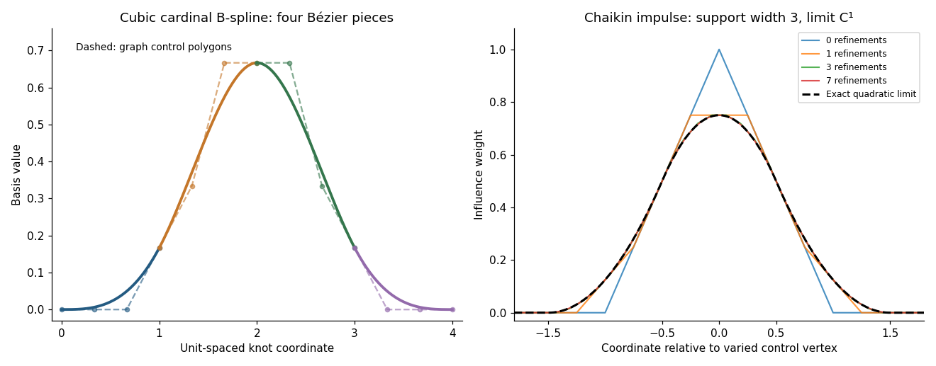
Four cubic B-spline Bézier pieces and the convergence of a Chaikin impulse to its quadratic basis function
. Details. 
A tensor-product surface basis combines two independent univariate bases:The coefficients are three-dimensional control points. Fixing one parameter gives a curve in the other univariate basis; the coefficients of that curve are the corresponding weighted combinations of rows or columns of controls.
The control net must have a rectangular two-index topology, with row/column neighbors and quadrilateral mesh cells. “Rectangular” describes the index grid, not the geometry of the points: its faces need not be flat or rectangular in space. A surface requiring a triangular domain or arbitrary extraordinary mesh connectivity is not directly described by one such tensor-product patch.
Let . Every available mixed derivative factors:If the univariate factors have continuity and , the right-hand side has equal one-sided traces across a knot for , and across a knot for . Their products therefore remain continuous, including where knot lines cross. The basis and its surface inherit coordinate-wise continuity orders , and joint continuity. In particular, degree- and degree- B-splines at simple knots give and continuity in the respective directions. Higher continuity can occur through special coefficient cancellation, but is not generally guaranteed.
Nonnegativity passes to products. Their partition of unity follows fromThus the surface remains in the convex hull of its active control points and commutes with application of affine functions. The support is the Cartesian product of the two univariate supports, giving local rectangular influence regions and efficient local evaluation. Linear precision also passes independently in each coordinate. Clamped endpoint interpolation gives boundary curves determined by the outer rows/columns and corner interpolation; parameter-line curves inherit the corresponding univariate properties. These are the relevant inherited properties, rather than a claim of arbitrary global variation-diminishing behavior for surfaces.
A triangular Bézier patch is a non-tensor-product example. On barycentric parameters with , defineThe indices satisfy a total-degree constraint, and couples the two independent parameters. The control net is triangular with points, rather than a rectangular product index set. The multinomial theorem gives nonnegative basis functions summing to one, but the entire basis is not a product of two independent univariate bases.
A parametric surface interrogation interface must specify its parameter domain, patch boundaries, trimming restrictions and any exceptional or singular points. It must evaluate and the available derivatives, in particular for tangent vectors andfor the oriented normal vector where the denominator is nonzero. Second derivatives are needed when the code requests curvature or second-order geometric error estimates; higher derivatives depend on the enquiry. The interface must report where these quantities exist, rather than assign an artificial normal at a singular parameter point.
Global searches also need subdivision into equivalent restricted patches, certified bounding volumes and a geometric approximation/error bound. These support intersection isolation, pruning and tolerance-controlled meshing. A single point-evaluation routine cannot guarantee a global search because it may miss remote branches or features between samples. Adjacent-patch topology and consistent orientation are needed to join results and interpret the represented surface.
Use the PDF's notation: is the fixed point light, is the casting curve, and is the receiver. A shadow point solvesThe separating-plane assumption puts the caster between light and receiver, so the relevant intersections are beyond the caster, not on the backward ray. The facing assumption supplies transverse regular intersections on the lit side. Carry out shadow tracing for a parametric curve as follows.
First subdivide the curve domain and receiving patches. Reject combinations whose certified bounding volumes cannot intersect the corresponding forward ray cone. For the remaining combinations, subdivide and isolate a hit, then correct its parameters using a three-variable Newton method with JacobianCheck that the corrected parameters lie in the patch domain and . Seed every connected component; one arbitrary initial hit does not establish that other components are absent. If a ray has several receiving hits, compare their values and retain the visible first hit, rather than jumping between sheets.
At a transverse branch the Jacobian is nonsingular because . Differentiate the equation to predict the next hit:Use this predictor for a proposed parameter step, then apply Newton correction. To control the polygonal approximation, the shadow path is . A second differentiation givesTogether with the surface derivatives this supplies a bound on . If over an interval of width , the maximum error from its chord is at most . Subdivide until this bound, plus the numerical intersection error, is below the graphics tolerance. Corrected endpoints then give the requested point sequence on . If second-derivative bounds are unavailable, refine until a certified enclosure of the entire branch segment lies within tolerance of its chord; a sufficiently small enclosure diameter is a conservative fallback.
Continue through adjacent patches, split at a trim or surface boundary, and stop a component when its admissible intersection ceases. Record closed components without duplicating their starting point. Use adaptive chord-error control and component isolation; a fixed fine sampling or an unverified sequence of local Newton solves can miss part of the shadow. If only estimated midpoint errors are available, those support a practical rendering heuristic rather than a certified tolerance.
Without the separation assumptions, explicitly test whether the caster lies between the light and receiver: roots with are not receiver points shadowed by that caster point, and belongs to the backward ray. The light can lie on the curve, making , or a ray can run along rather than cut the surface; both need exceptional treatment.
Without the facing assumption, allow back-facing regions, tangencies with singular continuation Jacobian, folds, multiple ray intersections, self-occlusion and changes of the visible first intersection. Visibility can create or delete whole shadow branches or switch them between receiver sheets. Also handle open boundaries, trimmed holes, disconnected receivers, closed casting loops, caster/receiver intersections and a light inside a closed receiver. Subdivision and intersection isolation must precede branch continuation near these events; normals, orientation and sorted ray distances decide which solutions are physically visible. The output can be several point sequences, rather than one connected polyline.
A subdivision surface interrogation interface needs the initial control net, its face/edge/vertex connectivity, the subdivision rule, patch addressing and refinement into child regions that cover the same limit surface. It must supply limit-point evaluation, available tangent/normal data and smoothness information, including the treatment of extraordinary subdivision vertices. A finite refined mesh point is generally not the exact limit point.
For geometric search it must provide certified bounding volumes for each descendant region, bounds that shrink under refinement, and a mesh-to-limit or chord/patch error estimate. With positive convex subdivision masks the active-control convex hull can provide such an enclosure; schemes with negative coefficients need another valid bound. A closed surface also needs consistent orientation, component navigation and containment queries for the enclosed body. The hypothesis supplies first-order tangent information at regular points, not automatically second derivatives or curvature everywhere. These enquiries distinguish an accurate limit-surface algorithm from a calculation only on an approximate control polyhedron.
Interpret the positive-distance assumption as disjoint compact enclosed bodies , certified for example by disjoint enclosing volumes. Merely having disjoint drawn control meshes is insufficient if one encloses the other or the meshes do not enclose their limit surfaces. For genuinely disjoint bodies, the closest pair lies on their boundaries: an interior point could move toward the other body and decrease the distance. Thus minimize over all pairs of limit-surface patches.
Use branch and bound on patch pairs. For regions , enclosing bounding volumes give a lower bound on their true minimum distance. For axis-aligned bounding boxes, compute this directly asAny pair of evaluated limit points provides a feasible upper bound; retain the smallest, . Start with a covering list of all coarse patch pairs. At each step, discard a pair when its lower bound is at least , otherwise refine the region with larger bounding diameter/error and enqueue its child pairs. Prefer the pair with smallest lower bound. Update with new feasible pairs; a local stationary-distance solve can improve it but cannot replace the global search.
Let be the minimum remaining lower bound, capped by if the list is empty. The current certificate isStop when . Compactness and shrinking valid patch enclosures ensure convergence to this tolerance under the interface assumptions. An equivalent mesh method must add each mesh's certified limit error; for Hausdorff distance errors , the separation error is at most . Finite mesh distance without such a bound is not the exact minimum distance between subdivision bodies.
First distinguish the ordinary set distance from a signed overlap convention. Ordinary is zero whenever the bodies intersect, and is never negative. Without the positive-separation assumption, test boundary intersections using the subdivision search, and test containment when the boundaries are disjoint. In particular, concentric spheres of unequal radii have positive boundary separation but overlapping enclosed bodies. Include every connected component in the containment tests.
For a meaningful negative result choose translational penetration depth, with orientation fixed:Define signed separation as ordinary positive distance for disjoint bodies, zero at contact, and when their interiors overlap. This is explicit; the source does not specify which penetration convention its word “distance” intends. Simply negating the closest-boundary distance fails when boundaries cross, because that distance is already zero despite genuine interior overlap.
One implementable extension searches translation space. Obtain an initial separating translation by moving beyond along a coordinate direction, using the bodies' enclosing boxes; its norm is an upper bound on . Cover a translation box containing the radius- ball, subdividing it into cells. Each cell has a lower bound on , given by its box distance from the origin. At a sampled translation, perform certified boundary-intersection and containment queries. A nonoverlapping sample improves .
To discard a whole colliding cell, certify an interior witness: if lies inside and lies inside with inward clearance , then every translation with still overlaps. Boundary-distance and inside tests establish this certificate. Conversely, a separated sample with clearance remains separated under translations of norm less than away from it, by the triangle inequality. For a wholly free cell, use its point nearest the origin as a feasible translation, attaining its cell-norm lower bound. Refine cells whose status is uncertain and whose minimum norm is below ; discard certified-colliding cells and irrelevant farther cells. Keep the minimum cell-norm bound among cells that might contain a separating translation as . Stop when , reportingRefinement/inside certificates can be implemented from the same surface hierarchy with conservative geometric bounds. Exact contact may require further refinement to decide topology; at finite numerical tolerance report a contact/uncertainty interval instead of inferring overlap from intersecting boxes. This handles crossing and containment and searches for the smallest separating translation, rather than an arbitrary visible intersection depth.
Articles by others on the same topic
There are currently no matching articles.