The input vector contains the activities of presynaptic units or sensory features, and contains the corresponding synaptic weights. The linear output is their weighted sum; it may be a centered activity proxy rather than a literal nonnegative spike rate. The learning time scale is , and take for normalization. The term is a Hebbian learning increment that strengthens weights correlated with the postsynaptic output. The term opposes unlimited growth.
For slow learning under stationary input statistics, average over inputs while holding the current weights fixed. Define . The averaged Oja's rule isIts squared norm obeysWhenever the output second moment is positive, this drives the norm toward , preventing the unbounded growth of an unconstrained Hebbian linear neuron. The direction becomes sensitive to dominant input correlations. Such a unit can learn a feature detector without supplied target labels, providing a simple mechanism for unsupervised learning and principal component analysis. This averaged analysis assumes input fluctuations are fast relative to learning; it is not a claim that every individual stochastic update follows the same deterministic trajectory.
For fixed weights during the input average,Thus is the input second-moment matrix. It is a positive semidefinite matrix because . If the inputs have been mean-centered, it is their covariance matrix; otherwise .
The stationary averaged learning equation isFor this makes an eigenvector of with eigenvalue . If , taking the inner product with givesand thereforeThe zero vector is also stationary but is not an eigenvector in the usual nonzero-vector definition. Likewise any vector in the nullspace of is stationary with zero output second moment and need not have the normalized length. These exceptional equilibria must be distinguished from a nonzero feature-learning solution.
Let be an orthonormal eigenbasis of , with . Expand . At the normalized length imposed on positive-output equilibria,Equality holds exactly when lies in the largest-eigenvalue eigenspace. If is simple,The norm constraint is essential: without it, scaling a direction with positive eigenvalue makes the output second moment arbitrarily large, so the printed maximization statement would have no finite maximum. When , this is the usual unit-length formulation.
For centered inputs, maximizing this quantity maximizes output variance. The unit therefore selects the first principal component analysis direction: a stimulus feature with the greatest variation in the input ensemble. Biologically, learned synaptic weights become selective to that dominant correlated pattern, rather than to a teacher-supplied label. For uncentered inputs it maximizes a second moment including the mean response, which is not the same as maximizing variance. If the top eigenvalue is repeated, any normalized vector in its eigenspace attains the same maximum.
Linearize the averaged rule about the genuine positive-eigenvalue equilibrium , where is a unit eigenvector. The question's unit-length hint implicitly uses ; for general the scaling is required. Put and . To first order,Substituting into the mean learning equation and cancelling the equilibrium terms gives stability and normalization of averaged Oja learning:In the eigenbasis, the radial and transverse perturbations satisfyFor , the radial direction contracts. Any nonmaximal eigenvector has a transverse direction with and is unstable. If and , both have strictly negative linearized eigenvalues and are locally asymptotically stable. Thus only the maximal-eigenvalue directions can be stable, with the usual simple-eigenvalue assumptions giving isolated attracting equilibria.
Convergence also needs an initial component along the top direction. For the full averaged equation, the coefficients obeyFor ,With a strict top eigenvalue, all other ratios tend to zero. The norm equation from part a then drives the nonzero weight norm to , so the weight converges to the top eigenvector with the sign of its initial top component. Random nonzero initialization has that component with probability one under a continuous distribution.
Several exceptions qualify the printed conclusion. A repeated largest eigenvalue gives neutral directions within the top eigenspace and convergence to a normalized vector in that space, not a unique eigenvector. An initial vector exactly orthogonal to the top eigenspace remains in that invariant subspace. The zero initialization stays zero. If , every weight is stationary and no distinguished component can be learned. Nonzero nullspace equilibria are unstable when has a positive eigenvalue. Hence unconditional convergence from every initial weight, or uniqueness without a spectral gap, would be false.
A visual neuron's receptive field specifies the region of visual space and stimulus features whose changes affect its response, with the surrounding and temporal context held appropriately controlled. A linear receptive-field approximation is a signed spatial weighting kernel. A simple cell in primary visual cortex commonly has elongated alternating ON and OFF subregions and orientation selectivity. Brightening an ON region increases its drive; darkening an OFF region does likewise, while opposite contrasts oppose that drive in the linear approximation.
The original sketch below uses a Gaussian-windowed cosine to depict an elongated ON strip with OFF flanks. A bar aligned with these regions can produce strong net drive, whereas an orthogonal bar produces more cancellation. This is an illustrative signed filter, not a claim that every simple cell has exactly this analytical shape.
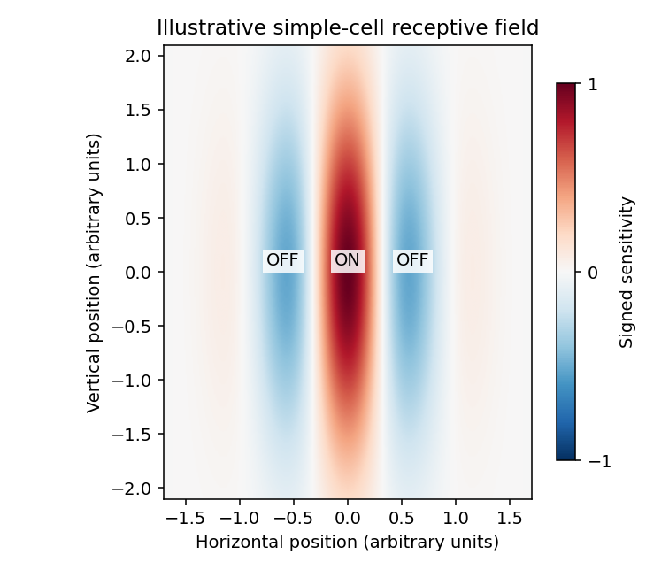
Illustrative simple-cell receptive field with elongated ON and OFF subregions
. Details. 
Different unsupervised learning models address different developmental aspects. Oja's rule can select a dominant direction of correlated input and provides normalization that a bare Hebbian update lacks. By itself, one linear principal component need not be localized, nor does it create a cortical map. Additional spatial constraints and competition are needed to explain a collection of spatially organized selective cells.
Competitive Hebbian learning among correlated ON and OFF inputs can separate those input types into adjacent subregions and generate orientation selectivity. Competition among inputs from the two eyes can similarly contribute to eye-specific preference and ocular dominance columns; spatial interactions between cortical units are needed for an organized map rather than merely one cell choosing one input pool. These models connect developmental organization to input correlations and normalization constraints. The ON/OFF competition model gives a concrete orientation-development example.
A different approach is sparse coding: learn features that reconstruct natural images while limiting simultaneous activity. This can yield localized, oriented, band-pass filters resembling simple-cell receptive fields, because it uses structure in natural-image statistics beyond the covariance alone. The original sparse-code model demonstrates this functional account. It does not by itself establish an exact developmental mechanism.
Correlated input, competition and normalization can produce selectivity; the objective and network constraints determine which aspect of cortical organization is explained. Anatomical constraints, spontaneous activity and experience must still be tested experimentally. A final receptive-field resemblance is weaker evidence than accurate predictions about its development and responses to altered input statistics.
Articles by others on the same topic
There are currently no matching articles.