An action potential is a brief regenerative change in a neuron's membrane potential, followed by repolarization and recovery. In a typical spiking neuron, depolarization recruits voltage-gated ion channels; inward current promotes further depolarization until inactivation and opposing currents terminate the event. The neuronal refractory period makes immediate repetition difficult or impossible. Once initiated, the roughly stereotyped event propagates along the axon. Its amplitude is therefore not generally the primary variable used to represent stimulus strength.
Inputs arriving at synapses on a neuron and its dendrites change membrane currents and produce graded voltage changes. Their spatial and temporal integration can trigger an action potential. At a chemical synapse, an arriving spike promotes release of a neurotransmitter, whose receptors alter the next neuron's conductances. Depending on the synapse and receptor mechanism, the input can promote or suppress the next neuron's firing. Thus information flows through activity patterns interacting with connectivity and synaptic dynamics, rather than by an identical voltage waveform simply passing unchanged across every cell.
In rate coding, a relevant response statistic is the number of spikes in a chosen interval, or the mean firing rate inferred from repeated trials or a population. For example, a sensory variable might be represented by mean counts of two versus five spikes in a ms window. A downstream neuron integrating many synaptic inputs over that window can distinguish the rates even if individual spike times vary. The window, averaging method and neuron's stimulus tuning must be specified; not every cell increases its rate for every stronger stimulus. Neural adaptation can also make the rate depend on recent stimulus history.
In temporal coding, precise times carry information beyond that count. Two responses containing the same number of spikes can differ in their first-spike latency after stimulus onset. Alternatively, spikes can lock to a particular phase of a periodic input, or relative timing across two neurons can encode coincidence. A decoder that reads only the long-window count discards those distinctions, whereas a temporally sensitive synapse or coincidence detector can use them.
Rate coding uses a chosen frequency or count summary; temporal coding uses the arrangement of spike times relative to a reference. They are complementary possibilities within neural coding, and a spike train can carry information in both. Stochastic variability does not prevent coding, but requires assessing how reliably different response distributions can be distinguished.
For a constant-rate Poisson process, let be the waiting time from a spike to the next spike. By independent increments, there is no spike in an interval of length with probability . Hence, for ,Its density is , so the interspike intervals are independent exponential distributions with mean . If is uniform on , inverse transform sampling gives . Repeatedly add independent draws to the current spike time to simulate a constant-rate spike train.
For a prescribed time-dependent nonnegative rate , use an Inhomogeneous Poisson process. Conditional on the present event at , its next waiting time has survival probabilityThus its conditional CDF is minus that expression for . Define the cumulative intensity . For each new independent uniform draw, set and solveThis transforms independent unit-rate exponential intervals in integrated-intensity time into physical spike times. Use a generalized inverse when the rate vanishes on an interval: no spikes are placed in a flat part of . On a finite simulation window, stop when the next intensity target exceeds the available . If the total future intensity is finite, a target beyond it means that no further spike occurs.
Numerically, integrate the known rate and invert the accumulated integral, or integrate exactly across piecewise-constant rate bins. Drawing an exponential interval using only is not exact when the rate changes during the interval. The Poisson model also omits the neuronal refractory period and other spike-history effects.
One useful starting point is reverse correlation, implemented as a spike-triggered average. Present a long stimulus record and retain the stimulus history before each observed spike. After subtracting the stimulus mean, estimatewhere is the number of spikes and is the history window. This identifies a candidate temporal receptive field. For white Gaussian stimulation and a one-filter encoding model, the average is proportional to the relevant filter, provided the response nonlinearity does not make that average vanish. For example an even response to the projection can have zero average despite strong stimulus dependence. Colored inputs require accounting for stimulus covariance, and more than one relevant stimulus direction may require a richer fitted model.
Use the candidate filter in an LNP model:Estimate the static nonlinearity by binning filter projections and dividing spike counts by exposure time in each bin. Equivalently, Bayes' rule gives under this model. Refine the filter and nonlinearity by maximizing the conditional Poisson log-likelihoodwith suitable regularization. Simulate an Inhomogeneous Poisson process at the fitted rate using integrated-intensity inversion from the previous solution. This gives a statistical encoding model, not a claim to reconstruct the neuron's ion channels.
Use cross-validation: estimate parameters on one set of trials and test them on independent held-out trials. Under repeated identical stimuli, compare the observed and simulated trial-averaged firing rates, spike-count distributions, interspike-interval distributions and autocorrelations. Compare held-out likelihoods and predictive errors with simpler baseline models and with the variability between real repeats. Exact spike-by-spike agreement is not expected from two independent realizations of a stochastic model. Large rate agreement accompanied by incorrect short-interval or correlation statistics reveals missing dynamics. Adding a spike-history term, for example in a point-process generalized linear model, can account for refractoriness or bursting when the basic Poisson cascade fails.
A good model predicts held-out response distributions, not just its training spike train. Such a model summarizes what stimulus features affect the neuron, permits controlled simulated changes of those features, and tests whether the proposed computation is sufficient. Its failures can suggest further experiments or additional stimulus and history variables.
Assume the two response labels are distinct and the error probability is the same for each stimulus. Then the stimulus-response map is a binary symmetric channel:with the two incorrect conditional probabilities equal to . Equal stimulus probabilities give . In bits, the Shannon entropy of the response is therefore . For either stimulus the response entropy is the binary entropywith . Thus , and the mutual information isIt is maximal, equal to one bit, at and also at . The latter response is always opposite to the ideal label but still specifies the stimulus perfectly after relabelling. It is minimal, equal to zero, at , when both response distributions are identical and the response is independent of the stimulus. If error is conventionally restricted to , the maximum occurs only at zero.
The symmetric-error assumption matters. A single overall error probability would not determine this information if the two stimuli had different conditional error rates or if the response included additional outcomes.
Computational models and biological experiments answer complementary questions. Experiments constrain what a nervous system actually does; a model makes a proposed explanation precise enough to test whether its mechanisms can produce those observations. The useful comparison is between competing, experimentally constrained explanations, rather than between modelling and experimentation as alternatives. A good model exposes assumptions, predicts new observations and identifies measurements that would distinguish it from rivals.
A Hodgkin-Huxley model links action potentials to voltage-dependent conductances and channel kinetics. It is more informative than merely fitting a spike waveform because changes in its conductances predict changes in excitability. Yet a model calibrated for one cell or preparation does not automatically represent another: different channel combinations and spatial geometry can yield similar outputs. Detailed parameters must be constrained by experiments, and apparent agreement does not make them uniquely identifiable. A leaky integrate-and-fire model deliberately sacrifices channel detail to study the effects of connectivity, timing and synapses in a large network. It is useful for such questions even though it cannot explain the microscopic origin of the action-potential waveform.
At a functional level, an LNP model tests which stimulus features predict a neuron's response and how those features map to firing rate. Independent testing, including response correlations rather than only mean rate, reveals what its assumptions miss. It can characterize a receptive field without claiming that the brain explicitly performs its particular fitted calculation. A Hopfield network likewise demonstrates that recurrent interactions can implement content-addressable memory: corrupted cues relax toward stored patterns. Its usefulness is an existence proof and a quantitative account of interference, not evidence that biological memory literally uses symmetric binary connections and the same update schedule.
Developmental models connect observed input statistics with synaptic plasticity. Hebbian learning with normalization or synaptic competition can produce selective weights and segregation of competing inputs. Models of correlated ON and OFF inputs can explain the formation of oriented simple-cell subregions and predict how changing the correlations changes their organization. That makes altered visual experience or patterned stimulation informative tests. Such models still need anatomical, developmental and plasticity constraints; several learning rules may reproduce similar final receptive fields. A primary model of activity-dependent ON/OFF competition illustrates this approach.
Normative models instead ask what representation would perform a specified task efficiently. For example, sparse coding of natural images can produce localized oriented filters resembling simple cell receptive fields. This links environmental statistics to a useful coding objective, but resemblance alone neither proves that the objective is the only explanation nor specifies the biological learning mechanism. Predictions about altered stimulus ensembles, population activity and synaptic changes provide stronger tests. The original sparse-code receptive-field model provides an example.
These distinctions also explain the dangers of models. Excessive flexibility can fit noise; unrealistic assumptions can generate a desired effect by construction; and multiple parameter sets can have nearly indistinguishable outputs. Simulation without analysis may obscure rather than explain a mechanism. Cross-validation, uncertainty analysis, comparisons with simpler models and controlled perturbations are therefore important. Conversely, collecting more measurements without a discriminating hypothesis can leave the same explanatory ambiguity unresolved.
The productive cycle is to propose a constrained model, determine which observations it predicts beyond the fitting data, perform the relevant experiment, and revise or reject the model. Models help select experiments and interpret results; experiments establish their scope and reveal omitted mechanisms. The appropriate level of detail depends on the question: spike-generation mechanisms, circuit computation and developmental organization need not be explained by the same model.
Interpret and as nonnegative firing-rate activities, rather than individual action potentials. Take . The relaxation time controls how quickly activity changes. The decay terms and make activity fall in the absence of recurrent drive. Each neuron receives a weighted input from the other, with coupling , and the static input-output function converts that input into a target activity.
The nonlinear response tends to at large input magnitude and equals at , so is its maximum activity and its half-saturation input scale. At small inputs it is approximately . For this is a mutually excitatory saturating rate network: increasing one neuron's activity increases the other's drive, permitting positive feedback. The response is even in , so this particular equation does not model a negative as ordinary inhibition; its dynamics depend on .
The equations combine passive relaxation with instantaneous nonlinear recurrent drive. They omit explicit spike timing, delays, channel dynamics and stochasticity, so they are an activity-level model for computational neuroscience.
Put . The nullclines areAny steady state has nonnegative coordinates because . For , is strictly increasing on the positive half-line. If a steady state had , then , a contradiction. The case is identical, so all steady states lie on the diagonal. Write . Besides , the equation givesand henceThus three distinct steady states exist exactly when , with and the positive parameter assumptions stated above. For positive excitatory coupling this is . At equality the two positive states merge; below it only the origin remains. If , the origin is again the only steady state.
Both nullclines begin at the origin and approach the limiting activity along their saturating direction; they are reflections of each other across . Flow points to the right where and to the left where . It points upwards where and downwards where . The plot shows these nullclines and typical trajectories for the parameters of the next part.
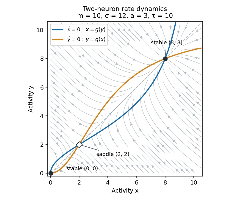

The origin and upper diagonal state attract nearby trajectories, while the lower positive state is a saddle. Its stable manifold separates the two attracting regions: trajectories in each basin of attraction approach its stable node, giving bistability. The diagonal is invariant, and on it the scalar activity increases between and and decreases between zero and or above . Activities remain nonnegative and bounded because . The vector field has constant negative divergence , so the Bendixson-Dulac criterion also rules out periodic orbits in the physical quadrant. The network is a switch between persistent activity levels, rather than an oscillator.
The Jacobian matrix at a diagonal steady state isIts eigenvectors and represent common and opposing perturbations, with respective eigenvalues and .
For a nonzero equilibrium, and . Consequently . The lower root has and is a saddle equilibrium; the upper root has and is a stable node. At the origin , so both eigenvalues are .
The supplied parameters give , and the nonzero roots solve , giving and . The numerical stability results areBiologically, the origin is a quiescent state and the upper equilibrium a sustained mutually reinforced activity state. The saddle represents a collective activation threshold: a perturbation crossing its basin boundary can switch the network from low to high activity. This persistent-state mechanism can model a memory or decision variable, but the simplified rate equations do not establish that a particular biological circuit uses it.
A standard binary Hopfield network contains recurrently connected units with activities . Choose symmetric weights , omit self-couplings by setting , and use zero thresholds for the energy in the next part. To store desired binary patterns , a simple choice is Hebbian memory weights for a Hopfield network:Correlated activity strengthens connections between units agreeing across the training patterns and makes disagreement contribute negatively. This creates attraction toward the stored configurations when cross-talk is sufficiently small. For one stored pattern, its local field is , so every bit is stable for . With multiple patterns, the other patterns add cross-talk; the rule does not guarantee exact retrieval for an arbitrary collection.
Start retrieval from a partial or corrupted cue and update one unit at a time using its current fieldA cyclic or random fair asynchronous schedule lets the network relax toward a fixed point, completing a memory when the cue lies in its basin. This is content-addressable retrieval: the initial pattern selects the memory without an explicit address. Nonzero thresholds can be included in a more general model, but their corresponding linear terms must then be included in the energy.
For the symmetric zero-diagonal weights and asynchronous rule just specified, update only unit . In the energy difference, terms involving neither nor its symmetric partner cancel. Thus asynchronous Hopfield energy descent givesIf the unit was already aligned, it does not change and . If it flips into alignment, , soAt our tie rule retains the old activity. The network has only configurations. Strict descent on every actual change prevents revisiting a configuration and permits only finitely many changes. With a fair schedule every misaligned unit is eventually updated, so the terminal configuration is a fixed point. At that point each possible single-bit flip has energy cost . The network reaches a minimum against single-unit changes, not necessarily the global minimum. Its energy is a Lyapunov function for these asynchronous dynamics.
The qualifications are essential to the printed claim. Synchronous updates can cycle: for two units with , the state alternates with , keeping energy . Symmetry alone therefore does not prove convergence under simultaneous updates.
Nor does the valid descent proof guarantee a global minimum. Consider four units with and all four cross-group weights equal to , symmetrically and with zero diagonal. The state has aligned fields and energy , so it is a strict single-flip local minimum. The all-positive state has energy . This explicit counterexample shows why local minima may trap retrieval even though the energy always descends under the stipulated rule.
One limitation is finite useful storage capacity and interference. Under simple Hebbian learning, each additional pattern contributes cross-talk to the retrieval fields; correlated or excessive patterns can erase a memory's basin or destabilize the pattern itself. More structured learning can reduce this interference: covariance-based weights account for activity biases, and pseudoinverse-based rules can orthogonalize a set of linearly independent patterns. Sparse representations and suitable thresholds can also change the capacity tradeoff. These extensions require their own retrieval analysis; they do not permit unlimited robust storage in a finite network.
A second limitation is spurious attractors and entrapment in unintended local minima. Mixtures of memories or unrelated configurations can be fixed points, and deterministic energy descent cannot escape an already stable incorrect state. Stochastic updates that sometimes accept energy increases can explore other configurations, and simulated annealing can gradually reduce that randomness to favor lower energies. Better weight learning and basin shaping can reduce the spurious states. Finite-temperature escape is probabilistic, and a practical finite-time annealing schedule does not guarantee the desired memory or a global minimum.
Changing the learning rule addresses interference; changing the retrieval dynamics can address trapping. The objective must still be appropriate: the lowest energy pattern is not necessarily the memory best matching a particular noisy cue.
The input vector contains the activities of presynaptic units or sensory features, and contains the corresponding synaptic weights. The linear output is their weighted sum; it may be a centered activity proxy rather than a literal nonnegative spike rate. The learning time scale is , and take for normalization. The term is a Hebbian learning increment that strengthens weights correlated with the postsynaptic output. The term opposes unlimited growth.
For slow learning under stationary input statistics, average over inputs while holding the current weights fixed. Define . The averaged Oja's rule isIts squared norm obeysWhenever the output second moment is positive, this drives the norm toward , preventing the unbounded growth of an unconstrained Hebbian linear neuron. The direction becomes sensitive to dominant input correlations. Such a unit can learn a feature detector without supplied target labels, providing a simple mechanism for unsupervised learning and principal component analysis. This averaged analysis assumes input fluctuations are fast relative to learning; it is not a claim that every individual stochastic update follows the same deterministic trajectory.
For fixed weights during the input average,Thus is the input second-moment matrix. It is a positive semidefinite matrix because . If the inputs have been mean-centered, it is their covariance matrix; otherwise .
The stationary averaged learning equation isFor this makes an eigenvector of with eigenvalue . If , taking the inner product with givesand thereforeThe zero vector is also stationary but is not an eigenvector in the usual nonzero-vector definition. Likewise any vector in the nullspace of is stationary with zero output second moment and need not have the normalized length. These exceptional equilibria must be distinguished from a nonzero feature-learning solution.
Let be an orthonormal eigenbasis of , with . Expand . At the normalized length imposed on positive-output equilibria,Equality holds exactly when lies in the largest-eigenvalue eigenspace. If is simple,The norm constraint is essential: without it, scaling a direction with positive eigenvalue makes the output second moment arbitrarily large, so the printed maximization statement would have no finite maximum. When , this is the usual unit-length formulation.
For centered inputs, maximizing this quantity maximizes output variance. The unit therefore selects the first principal component analysis direction: a stimulus feature with the greatest variation in the input ensemble. Biologically, learned synaptic weights become selective to that dominant correlated pattern, rather than to a teacher-supplied label. For uncentered inputs it maximizes a second moment including the mean response, which is not the same as maximizing variance. If the top eigenvalue is repeated, any normalized vector in its eigenspace attains the same maximum.
Linearize the averaged rule about the genuine positive-eigenvalue equilibrium , where is a unit eigenvector. The question's unit-length hint implicitly uses ; for general the scaling is required. Put and . To first order,Substituting into the mean learning equation and cancelling the equilibrium terms gives stability and normalization of averaged Oja learning:In the eigenbasis, the radial and transverse perturbations satisfyFor , the radial direction contracts. Any nonmaximal eigenvector has a transverse direction with and is unstable. If and , both have strictly negative linearized eigenvalues and are locally asymptotically stable. Thus only the maximal-eigenvalue directions can be stable, with the usual simple-eigenvalue assumptions giving isolated attracting equilibria.
Convergence also needs an initial component along the top direction. For the full averaged equation, the coefficients obeyFor ,With a strict top eigenvalue, all other ratios tend to zero. The norm equation from part a then drives the nonzero weight norm to , so the weight converges to the top eigenvector with the sign of its initial top component. Random nonzero initialization has that component with probability one under a continuous distribution.
Several exceptions qualify the printed conclusion. A repeated largest eigenvalue gives neutral directions within the top eigenspace and convergence to a normalized vector in that space, not a unique eigenvector. An initial vector exactly orthogonal to the top eigenspace remains in that invariant subspace. The zero initialization stays zero. If , every weight is stationary and no distinguished component can be learned. Nonzero nullspace equilibria are unstable when has a positive eigenvalue. Hence unconditional convergence from every initial weight, or uniqueness without a spectral gap, would be false.
A visual neuron's receptive field specifies the region of visual space and stimulus features whose changes affect its response, with the surrounding and temporal context held appropriately controlled. A linear receptive-field approximation is a signed spatial weighting kernel. A simple cell in primary visual cortex commonly has elongated alternating ON and OFF subregions and orientation selectivity. Brightening an ON region increases its drive; darkening an OFF region does likewise, while opposite contrasts oppose that drive in the linear approximation.
The original sketch below uses a Gaussian-windowed cosine to depict an elongated ON strip with OFF flanks. A bar aligned with these regions can produce strong net drive, whereas an orthogonal bar produces more cancellation. This is an illustrative signed filter, not a claim that every simple cell has exactly this analytical shape.
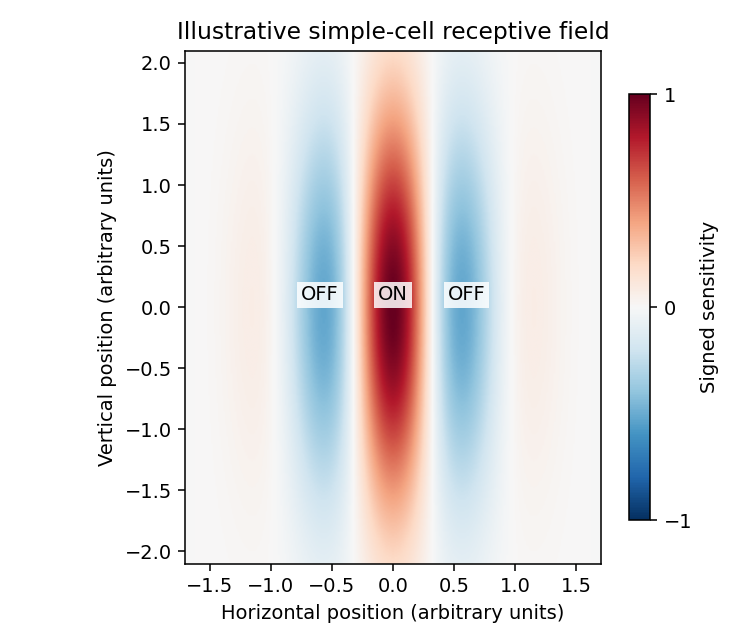
Illustrative simple-cell receptive field with elongated ON and OFF subregions
. Details. 
Different unsupervised learning models address different developmental aspects. Oja's rule can select a dominant direction of correlated input and provides normalization that a bare Hebbian update lacks. By itself, one linear principal component need not be localized, nor does it create a cortical map. Additional spatial constraints and competition are needed to explain a collection of spatially organized selective cells.
Competitive Hebbian learning among correlated ON and OFF inputs can separate those input types into adjacent subregions and generate orientation selectivity. Competition among inputs from the two eyes can similarly contribute to eye-specific preference and ocular dominance columns; spatial interactions between cortical units are needed for an organized map rather than merely one cell choosing one input pool. These models connect developmental organization to input correlations and normalization constraints. The ON/OFF competition model gives a concrete orientation-development example.
A different approach is sparse coding: learn features that reconstruct natural images while limiting simultaneous activity. This can yield localized, oriented, band-pass filters resembling simple-cell receptive fields, because it uses structure in natural-image statistics beyond the covariance alone. The original sparse-code model demonstrates this functional account. It does not by itself establish an exact developmental mechanism.
Correlated input, competition and normalization can produce selectivity; the objective and network constraints determine which aspect of cortical organization is explained. Anatomical constraints, spontaneous activity and experience must still be tested experimentally. A final receptive-field resemblance is weaker evidence than accurate predictions about its development and responses to altered input statistics.
Articles by others on the same topic
There are currently no matching articles.