For the binomial branching process, the offspring probability generating function is . The Galton-Watson extinction fixed point gives .
The printed finite-binomial upper bound is false without an additional asymptotic qualification. For and , solving the fixed-point equation exactly givesFor instance gives . More generally, at every fixed the Taylor expansion gives , again contradicting that upper bound for sufficiently small positive .
Here is the corrected binomial branching survival correction. The Poisson branching process of mean has branching survival probability satisfying . Expanding the logarithm givesThus , which implies the requested lower estimate . Since on , iteration of the two offspring probability generating functions gives .
For the actual binomial branching process, expansion of its exact fixed-point equation givesIf , all coefficients are nonnegative. Keeping the first term provesIn particular, for and this gives . The printed bounds also hold for the binomial branching process in an explicit large- regime: and . Indeed these conditions give and . In the preceding nonnegative series, evaluation at givesThe series is increasing, and its value at the actual branching survival probability is , so . Together with the lower bound already proved, this recovers in that regime. In particular it applies eventually to part (ii). The counterexample shows why a regime condition is needed for a literal finite- statement.
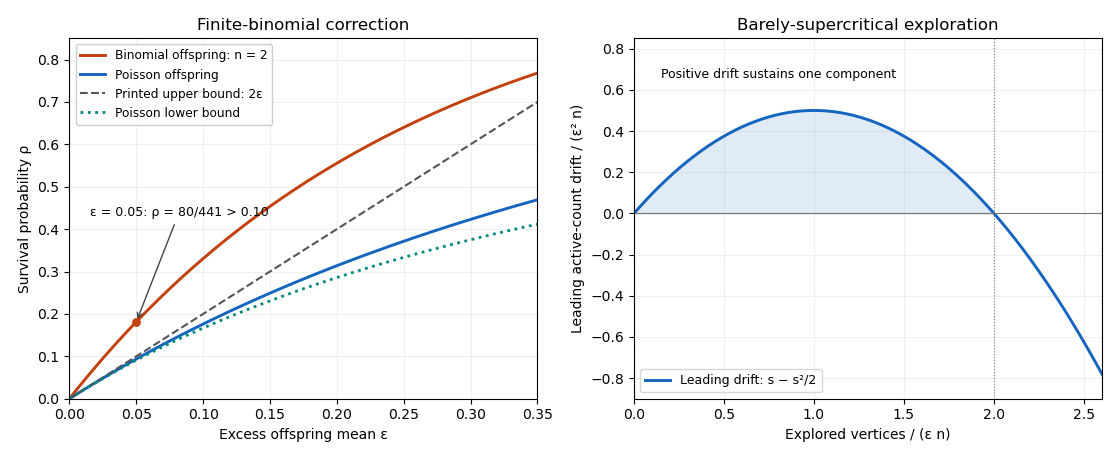
Finite-binomial survival exceeds the printed upper bound, while Poisson survival lies between the corrected comparison bounds
. Details. 
Write , , , and let be the total progeny of a binomial branching process. The preceding binomial branching survival correction gives . For a branching process conditioned on extinction, the offspring probability generating function is , with meanfor sufficiently large . Summing expected generation sizes therefore gives .
Put and let count vertices in graph components of order at least . A breadth-first exploration of a binomial random graph is dominated by . The Markov inequality applied to finite total progeny givesAlways . Since , we have and . Hence . This bound controls the expected value directly, including rare large graph components.
For the lower bound, use the breadth-first exploration of a binomial random graph with unseen vertices, active vertices and explored vertices, starting from , . Let indicate a new root. Conditional on the past, the newly discovered count has a binomial distribution . Put . The unseen-count recursion givesHere is a martingale. Up to , martingale-difference orthogonality gives , since each conditional variance is at most and is bounded.
Take . Then , and . The Doob L2 maximal inequality impliesThe Taylor expansion, uniformly for , gives . Thus throughout the integer interval for large . The new-root sum is nonnegative, so on the preceding event throughout this interval. No graph component finishes there: all these explored vertices belong to one graph component, of order at least , with high probability. Its expected value is therefore at least . Combining both inequalities provesThe barely-supercritical largest-component expectation uses both a positive exploration window and a finite-progeny bound; a bare convergence-in-probability assertion would not by itself justify this expectation.
Articles by others on the same topic
There are currently no matching articles.