Past exam of the mathematics course of the University of Cambridge / 2014 / iii / Paper 32 / 2

There are three free transition intensities: progression, death from the initial state, and death from the advanced state. In the three-state illness-death model, state 3 is an absorbing state, and there is no recovery transition.

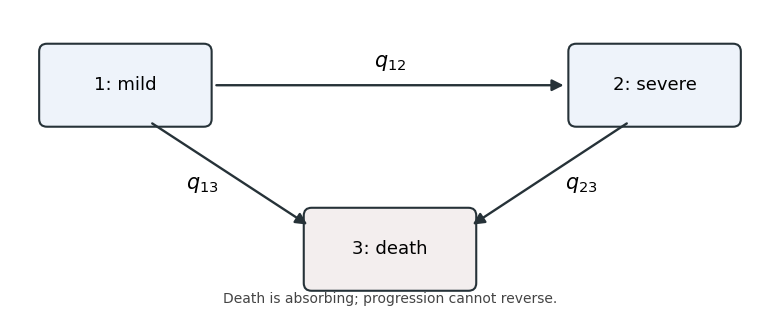
Writing $a=q_{12}$, $b=q_{13}$ and $c=q_{23}$, with all three nonnegative, the transition intensity matrix isEach diagonal entry is minus the sum of the row's outgoing transition intensities, rather than an additional unknown parameter. A continuous-time multi-state model with these rates describes the severity labels in the observations; an explicit cured state would require a richer state space.

In a time-homogeneous continuous-time Markov chain, a state's holding time is exponential with rate equal to its total outgoing transition intensity. Converting the specified times to months givesThe exit-type probability follows by dividing its transition intensity by the total exit rate. ThereforeThese are starting values for numerical estimation, rather than further observations or constraints on the final fitted rates.

Let $p_{rs}(t)=P(X(u+t)=s\mid X(u)=r)$ and $P(t)=e^{Qt}$, where time homogeneity removes dependence on $u$. A recorded state at the next clinic visit contributes a transition probability; an exactly observed death contributes a statistical probability density, not the probability of being dead at that time. If the last recorded living state is $r$, the mixed panel and exact-death likelihood factor after an interval $t$ isThis sums over the unobserved living state immediately before death.

Conditioning on the recorded initial states, the contribution of the three displayed patient histories isIn this irreversible illness-death model, $p_{21}=0$, $p_{11}(t)=e^{-(a+b)t}$ and $p_{22}(t)=e^{-ct}$, simplifying it toThe factor $c$ is essential: the death time is known exactly. Replacing the final statistical probability density by $p_{23}(34.6)$ would instead model interval observation of death and give a different likelihood.

The assumptions are independent patient histories with common rates; the Markov property; constant rates over calendar/follow-up time in this model; the stated absence of recovery and absorption at death; accurate state labels and death times; and an observation/follow-up mechanism that is noninformative for the latent process given the observed history. Clinic dates are conditioned on. The displayed living endpoints contribute only the shown observations, with noninformative right censoring if they are follow-up endpoints. Initial state probabilities are omitted by conditioning on them. Progression between visits can be unobserved, which is precisely why panel-observed multi-state likelihood uses the matrix exponential rather than assuming a transition occurs at a visit.

The mean holding time from a transition intensity matrix is $-1/q_{rr}$. Apply this to the fitted exit rates and use monotonic inversion for each confidence interval:Thus the expected state durations are 86.96 months and 31.45 months, respectively. A confidence interval for a reciprocal rate reverses the endpoint order; the negative diagonal rates must first be converted to positive exit rates.

For the expected absorption time in an illness-death model, the time spent initially in the mild state is followed by an additional severe-state duration only if progression occurs before death. That probability is $0.0072/0.0115$. ThereforeThis is an unconditional mean including both possible paths to death, not a mean conditional on progression.

In the log-linear transition intensity model, each hazard ratio multiplies a specific off-diagonal transition intensity, comparing its post-transplant period with the pre-transplant period while holding the modeled origin state fixed. Diagonal entries must then be recalculated from row sums.

For mild-to-severe progression, the early hazard ratio $0.52$ suggests a 48% decrease, but its interval $(0.11,2.4)$ includes no effect. The later hazard ratio $0.02$, with interval wholly below one, suggests a 98% decrease. These findings are compatible with suppression of progression by hematopoietic stem cell transplantation among those remaining in the mild state.

For mild-to-death, the early hazard ratio $43.92$ indicates a very large relative increase, and the later ratio $3.54$ still indicates an increase; both intervals are above one. For severe-to-death, the early ratio $2.37$ indicates increased mortality, whereas the later ratio $0.57$ indicates a 43% decrease; these intervals also exclude one. Early treatment toxicity and infection are plausible explanations for an immediate mortality increase. Later control of the underlying myelodysplastic syndrome is a plausible explanation for reduced advanced-state mortality and progression.

Relative increases must be interpreted alongside baseline rates. The early mild-state death rate is approximately $0.0016\times 43.92=0.0703$ per month, whereas the early severe-state death rate is $0.0380\times 2.37=0.0901$ per month. Thus the far larger mild-state hazard ratio partly reflects its much smaller starting mortality, rather than greater absolute mortality after transplantation. The later corresponding rates are $0.00566$ and $0.02166$ per month.

Within the question's model, delaying transplantation while the disease is mild can avoid a large immediate mortality cost, whereas the high baseline mortality in the severe state makes the later survival benefit more valuable. This provides a qualitative rationale for the stated policy. The estimates do not establish an optimal timing rule: treatment selection, changing health status, selection of survivors into the later period and the use of the previous visit's covariate value can affect the comparison. They are associations from the fitted cohort model, not automatically causal hazard ratios.