Past exam of the mathematics course of the University of Cambridge / 2014 / iii / Paper 32 (Biostatistics)

For a one-sided Wald test use the signed normal Wald statistic, rather than its square. The maximum-likelihood estimate is the sample mean ${\bar{Y}}_n$, with exact variance ${\sigma }^2/n$, soA sum of independent normal random variables is normal, giving ${\bar{Y}}_n\sim N(\delta ,{\sigma }^2/n)$ and hence $W_n\sim N(\sqrt{n}\delta /\sigma ,1)$. Under the null hypothesis its mean is zero:Thus its null distribution is exactly the standard normal distribution, without an asymptotic approximation. If the squared Wald statistic convention is used, $W_n^2$ has a chi-squared distribution with one degree of freedom; the signed form is needed to distinguish the two directions.

The same affine transformation of the normal distribution givesIts variance stays one while its mean moves positively. This is the exact alternative distribution used to calculate statistical power. The square, if used instead, has a noncentral chi-squared distribution with one degree of freedom and noncentrality $n({\delta }^{\ast }{)}^2/{\sigma }^2$.

Let $z_p={\Phi }^{-1}(p)$ denote a quantile of the standard normal distribution. Reject when $W_n>z_{1-\alpha }$. The statistical power at the specified positive effect isEquating this to $1-\beta$ and using $z_{\beta }=-z_{1-\beta }$ gives $\sqrt{n}{\delta }^{\ast }/\sigma =z_{1-\alpha }+z_{1-\beta }$. Thus, for the usual target $1-\beta >\alpha$,Rounding up ensures at least the target statistical power. This normal-mean sample size calculation assumes a positive integer sample size; if a requested power is at most $\alpha$, every positive sample size already exceeds that target for ${\delta }^{\ast }>0$, and one should not square a negative quantile sum to impose an unnecessary lower bound.

Write $s=\sigma /\sqrt{n}$, $\mu =\delta /s$, and let $Z_1,Z_2$ be independent standard normal random variables obtained by centering and scaling the separate stage means. ThenThe second statistic uses all patients, so the statistics are correlated even though the stages' new observations are independent. Their covariance is $1/\sqrt{2}$ and each variance is one. This gives the exact bivariate normal distributionUnder the null hypothesis both means are zero. At $\delta ={\delta }^{\ast }$ replace $\mu$ by $\sqrt{n}{\delta }^{\ast }/\sigma$; the mean vector is $(\sqrt{n}{\delta }^{\ast }/\sigma ,\sqrt{2n}{\delta }^{\ast }/\sigma {)}^T$. In this group sequential design the full-sample statistic may be viewed as a potential statistic from the underlying sequence of outcomes, even on paths where recruitment stops.

Set $z=z_{1-\alpha }$. Under the null hypothesis rejection requires both $W_1\ge f$ and $W_2>z$. Since $W_2$ has the standard normal distribution,The bivariate normal distribution in the preceding calculation has a nonsingular covariance matrix and strictly positive statistical probability density everywhere. For every finite futility boundary $f$ and $0<\alpha <1$, the open rectangle $\{W_1<f,W_2>z\}$ has positive probability. ThereforeFor an explicit expression, conditional on $W_1=w$ the full-sample statistic is $N(w/\sqrt{2},1/2)$ under the null hypothesis, yieldingThe Type I error is reduced because some otherwise rejecting paths stop for futility. Equality is approached as $f\to -\infty$, but does not hold at a finite futility boundary.

Let $X$ and $Y$ denote the first- and second-stage sample means, let $s=\sigma /\sqrt{n}$, and write $S=(X+Y)/2$. Continuation is the selection event $\mathcal{C}=\{X\ge sf\}$. The second-stage sample mean stays independent of $\mathcal{C}$, so $E(Y\mid \mathcal{C})=\delta$. The first-stage sample mean has a truncated normal distribution. With $a=f-\delta /s$ and the upper-tail Inverse Mills ratio $\lambda (a)=\varphi (a)/(1-\Phi (a))$,The positive conditional selection bias after futility continuation comes from selecting unusually large first-stage outcomes. The unconditional sample mean of a fixed $2n$ observations would be unbiased; that is a different sampling distribution from the one restricted to continued trials.

As $\delta \to \infty$, $a\to -\infty$, $\varphi (a)\to 0$ and $1-\Phi (a)\to 1$, so the estimator bias tends to zero. It decreases with $\delta$: differentiating gives ${\lambda }^{\prime }(a)=\lambda (a)(\lambda (a)-a)>0$, because $\lambda (a)=E(Z\mid Z>a)>a$ for a standard normal random variable. Thus

Use a Rao-Blackwell estimator after interim selection, which is exactly conditionally unbiased. The second-stage sample mean $Y$ alone is unbiased conditional on continuation, but discards the earlier observations. Apply the Rao-Blackwell theorem by averaging $Y$ conditional on the combined sample mean $S$ and the fact of continuation.

Set $c=sf$ and $v=s/\sqrt{2}=\sigma /\sqrt{2n}$. Before truncation, $X\mid S$ is $N(S,v^2)$, a distribution whose mean no longer involves the unknown $\delta$. After imposing $X\ge c$, its mean is $S+v\lambda ((c-S)/v)$. Since $Y=2S-X$, the resulting estimator isIt uses the outcomes from both stages through their combined sample mean. By iterated expectation, $E(\tilde{\delta }\mid \mathcal{C})=E(Y\mid \mathcal{C})=\delta$, so its conditional estimator bias is zero, compared with the strictly positive estimator bias above. Its conditional variance is no larger than that of the second-stage-only estimate. This does not assert a smaller mean squared error than every biased estimator.

There are three free transition intensities: progression, death from the initial state, and death from the advanced state. In the three-state illness-death model, state 3 is an absorbing state, and there is no recovery transition.

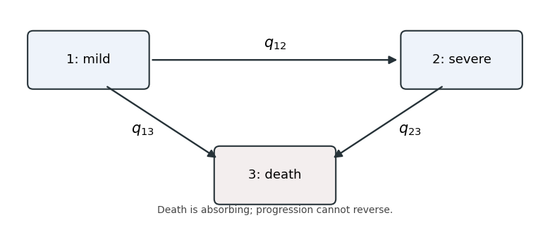
Writing $a=q_{12}$, $b=q_{13}$ and $c=q_{23}$, with all three nonnegative, the transition intensity matrix isEach diagonal entry is minus the sum of the row's outgoing transition intensities, rather than an additional unknown parameter. A continuous-time multi-state model with these rates describes the severity labels in the observations; an explicit cured state would require a richer state space.

In a time-homogeneous continuous-time Markov chain, a state's holding time is exponential with rate equal to its total outgoing transition intensity. Converting the specified times to months givesThe exit-type probability follows by dividing its transition intensity by the total exit rate. ThereforeThese are starting values for numerical estimation, rather than further observations or constraints on the final fitted rates.

Let $p_{rs}(t)=P(X(u+t)=s\mid X(u)=r)$ and $P(t)=e^{Qt}$, where time homogeneity removes dependence on $u$. A recorded state at the next clinic visit contributes a transition probability; an exactly observed death contributes a statistical probability density, not the probability of being dead at that time. If the last recorded living state is $r$, the mixed panel and exact-death likelihood factor after an interval $t$ isThis sums over the unobserved living state immediately before death.

Conditioning on the recorded initial states, the contribution of the three displayed patient histories isIn this irreversible illness-death model, $p_{21}=0$, $p_{11}(t)=e^{-(a+b)t}$ and $p_{22}(t)=e^{-ct}$, simplifying it toThe factor $c$ is essential: the death time is known exactly. Replacing the final statistical probability density by $p_{23}(34.6)$ would instead model interval observation of death and give a different likelihood.

The assumptions are independent patient histories with common rates; the Markov property; constant rates over calendar/follow-up time in this model; the stated absence of recovery and absorption at death; accurate state labels and death times; and an observation/follow-up mechanism that is noninformative for the latent process given the observed history. Clinic dates are conditioned on. The displayed living endpoints contribute only the shown observations, with noninformative right censoring if they are follow-up endpoints. Initial state probabilities are omitted by conditioning on them. Progression between visits can be unobserved, which is precisely why panel-observed multi-state likelihood uses the matrix exponential rather than assuming a transition occurs at a visit.

The mean holding time from a transition intensity matrix is $-1/q_{rr}$. Apply this to the fitted exit rates and use monotonic inversion for each confidence interval:Thus the expected state durations are 86.96 months and 31.45 months, respectively. A confidence interval for a reciprocal rate reverses the endpoint order; the negative diagonal rates must first be converted to positive exit rates.

For the expected absorption time in an illness-death model, the time spent initially in the mild state is followed by an additional severe-state duration only if progression occurs before death. That probability is $0.0072/0.0115$. ThereforeThis is an unconditional mean including both possible paths to death, not a mean conditional on progression.

In the log-linear transition intensity model, each hazard ratio multiplies a specific off-diagonal transition intensity, comparing its post-transplant period with the pre-transplant period while holding the modeled origin state fixed. Diagonal entries must then be recalculated from row sums.

For mild-to-severe progression, the early hazard ratio $0.52$ suggests a 48% decrease, but its interval $(0.11,2.4)$ includes no effect. The later hazard ratio $0.02$, with interval wholly below one, suggests a 98% decrease. These findings are compatible with suppression of progression by hematopoietic stem cell transplantation among those remaining in the mild state.

For mild-to-death, the early hazard ratio $43.92$ indicates a very large relative increase, and the later ratio $3.54$ still indicates an increase; both intervals are above one. For severe-to-death, the early ratio $2.37$ indicates increased mortality, whereas the later ratio $0.57$ indicates a 43% decrease; these intervals also exclude one. Early treatment toxicity and infection are plausible explanations for an immediate mortality increase. Later control of the underlying myelodysplastic syndrome is a plausible explanation for reduced advanced-state mortality and progression.

Relative increases must be interpreted alongside baseline rates. The early mild-state death rate is approximately $0.0016\times 43.92=0.0703$ per month, whereas the early severe-state death rate is $0.0380\times 2.37=0.0901$ per month. Thus the far larger mild-state hazard ratio partly reflects its much smaller starting mortality, rather than greater absolute mortality after transplantation. The later corresponding rates are $0.00566$ and $0.02166$ per month.

Within the question's model, delaying transplantation while the disease is mild can avoid a large immediate mortality cost, whereas the high baseline mortality in the severe state makes the later survival benefit more valuable. This provides a qualitative rationale for the stated policy. The estimates do not establish an optimal timing rule: treatment selection, changing health status, selection of survivors into the later period and the use of the previous visit's covariate value can affect the comparison. They are associations from the fitted cohort model, not automatically causal hazard ratios.

Let $Y$ denote the full data and $R$ the pattern of indicators, with $R_j=1$ for an observed component and $R_j=0$ for a missing one. For each fixed pattern $r$, split the data as $y=(y_{\mathrm{obs}}(r),y_{\mathrm{mis}}(r))$. The missing at random condition isHere $\psi$ parameterizes the missingness mechanism. Equivalently its conditional probability, with the observed data fixed, is constant over all possible completions of the missing data. The restriction is pattern-specific because the observed components depend on $r$. Missing at random allows missingness to depend on observed values; missing completely at random imposes independence from all the data.

Ask the doctor whether, among patients with the same first-year drug-use status, patients who dropped out would be more or less likely to have used the drug in the second year than those who remained. The comparison is within the observed first-year categories, not just between all dropouts and all completers.

If there is no remaining relationship with second-year drug use after conditioning on first-year use, missing at random is plausible for these recorded variables. If treatment-related difficulties, new medication or deterioration lead to dropout in a way not accounted for by the recorded first-year status, missing at random may fail. A different response rate in the two first-year categories is allowed under missing at random. The unobserved second-year outcomes mean that the observed table alone cannot establish this assumption; clinical knowledge or additional follow-up information is needed.

Apply MAR standardization over a fully observed covariate. All first-year statuses are known, so the estimated probabilities of no use and use in year one are $58/102$ and $44/102$. Within those categories, missing at random lets the observed second-year probabilities represent the corresponding dropout outcomes as well. They are estimated by $7/37$ and $18/28$.

The law of total probability then givesEquivalently, impute expected drug-use counts $21(7/37)$ and $16(18/28)$ for the two dropout groups, add these to the 25 observed second-year users, and divide by 102. This uses both the complete records and the fully observed first-year information.

Under missing completely at random, the observed second-year outcomes form a random subsample, so the direct pooled complete-case analysis estimate isIt is valid under missing completely at random because dropout no longer changes the marginal distribution of second-year use. Pooling is simpler than reporting separate conditional probabilities, but MCAR alone does not make this estimate more efficient than the estimate in the previous part. The fully observed first-year variable carries useful outcome information and can improve precision even when dropout is completely random.

To make the qualification explicit, write $X=Y_1$, $m(X)=P(Y_2=1\mid X)$, $\theta =E\{m(X)\}$ and $\rho =P(R=1)$ for the constant response probability. For $N$ patients the leading variance of the pooled estimator is $\mathrm{Var}(Y_2)/(N\rho )$. The standardization estimator in the preceding part has leading varianceIndeed its first-order centered contribution is $m(X)-\theta +R\{Y_2-m(X)\}/\rho$: the two terms have zero covariance, and their variances give that expression. The law of total variance therefore yieldsThe inequality is strict when there is dropout and first-year use predicts second-year use, as the distinct conditional rates suggest here. Thus the requested universal efficiency claim needs qualification. In the unrestricted joint binary-outcome model, maximizing the observed-data likelihood under either missing at random or missing completely at random gives the same standardization estimate $0.384889$: the all-patient first-year proportion and the two observed conditional second-year proportions maximize its factored outcome likelihood. Restricting the distinct missingness parameters to a common response probability affects their factor, not this estimate. The pooled value is the simple valid MCAR answer; retaining the first-year information gives the efficient MCAR answer and does not require replacing the previous estimate.

An ignorable missingness mechanism need not be absent from the data-generating process. It means that likelihood inference about the data-model parameters can omit the missingness factor, while still integrating over missing values.

Write the complete joint data statistical probability density as $f_{\theta }(y,x)$ and the conditional missingness probability as $g_{\psi }(r\mid y,x)$. All $y$ values and only $x_{\mathrm{obs}}$ are observed. Under missing at random, $g_{\psi }(r\mid y,x)$ is constant as $x_{\mathrm{mis}}$ varies with $(y,x_{\mathrm{obs}})$ fixed. The actual observed-data likelihood is thereforeThe assumed distinctness is understood as independent variation of $\theta$ and $\psi$. Maximizing over $\psi$ multiplies $L_{\mathrm{obs}}$ by a factor independent of $\theta$; likelihood ratios, scores and likelihood curvature for $\theta$ are therefore unchanged by omitting $g_{\psi }$. This proves likelihood ignorability.

For implementation of the observed-data likelihood with a missing covariate, a linear regression model for $Y\mid X$ must be accompanied by an appropriate model for the distribution of $X$. For independent individuals, write $f_{\beta }(y\mid x)$ for the regression statistical probability density and $g_{\eta }(x)$ for the age statistical probability density. Up to the ignorable factor,Ignorability does not authorize discarding missing-age cases or assuming their ages have the distribution seen in the complete cases. It removes the need to model the observation mechanism for likelihood inference under the stated conditions, not the need to handle the missing covariates.

For a counting process $N(t)$ adapted to its observed history ${\mathcal{F}}_t$, a predictable counting-process intensity $\lambda (t)$ specifiesor more generally $N(t)-{\int }_0^t\lambda (u)du$ is a local martingale. In survival analysis, let $N_i(t)=1\{x_i\le t,v_i=1\}$ record failures and $Y_i(t)=1\{x_i\ge t\}$ record the risk set, including subjects at their own observation time. Under independent right censoring and a common hazard function $h$, the aggregate intensity is $Y(t)h(t)$, where $N={\sum }_i{N}_i$ and $Y={\sum }_i{Y}_i$.

Writing $H(t)={\int }_0^{t}h(u)du$, the conditional increment equation is $E(dN\mid {\mathcal{F}}_{t-})=YdH$. Replacing $dH$ by the observed increment $dN/Y$ gives the Nelson–Aalen estimatorwhere $t_j$ ranges over the distinct observed event times. Censored observations remove subjects from subsequent risk sets but do not produce hazard jumps.

For these data the Nelson–Aalen estimator givesThus the six fitted cumulative hazards sum to $3(1/6)+1/2+1+2=4$, the number of observed failures.

The event-count identity for Nelson–Aalen cumulative hazards follows by exchanging the finite sums. With everyone entering at time zero,This includes each failure subject in its own risk set. A delayed-entry dataset requires a different risk indicator and is not covered by this particular identity.

Under a constant hazard survival model, $\hat{H}(x_i)=\hat{\theta }{x}_i$. Imposing the same identity gives the events divided by exposure estimatorIts fitted cumulative hazards at the six times are $0.3,0.4,0.5,0.6,0.9,1.3$, again summing to four. It is also the maximum-likelihood estimate under independent right censoring, since the parameter-dependent likelihood is ${\theta }^d{e}^{-\theta {\sum }_i{x}_i}$. This is a sensible estimate if the exponential survival model is appropriate, but four failures give little precision. The event-count identity by itself does not validate constant hazard; the large final jump in the Nelson–Aalen estimator also reflects a risk set of one, rather than by itself proving an increasing hazard.

For a proper continuous event time, the survival function is $S(t)=e^{-H(t)}$. The assumed invertibility of the cumulative hazard function gives, for $u\ge 0$,ThereforeThis is the cumulative hazard probability transformation; it applies also conditionally on a subject's covariates, using that subject's correctly specified cumulative hazard function.

The fitted transformed times are Cox–Snell residuals. They retain their event/right censoring indicators, so a right-censored residual represents an exponential observation known only to exceed its displayed value. Under the fitted model and independent right censoring, calculate the Kaplan–Meier estimator of residual survival and compare it with $e^{-y}$, or calculate the residual Nelson–Aalen estimator and compare its cumulative hazard with the diagonal $H(y)=y$. Systematic departures reveal model inadequacy; sparse extreme residual risk sets and parameter estimation require caution. Treating all censored residuals as observed event times would invalidate this diagnostic.

Without right censoring, the residual mean should be approximately one. With right censoring, use the modified Cox–Snell residualFor a true unit-rate exponential distribution, the memoryless property gives $E(U\mid U>c)=c+1$. Thus an event keeps its known transformed time, while a censored observation is replaced by the conditional expected event time. Under independent right censoring, iterated expectation makes the mean of these adjusted values one when the true hazards are used, and approximately one when fitted hazards are used. These mean-imputed values do not themselves have an exponential distribution, so the survival-curve diagnostic should still use the original censored residual dataset. Moreover fitting equations can force the adjusted sample mean to one, making its mean alone a weak diagnostic.

For the proposed mixture of a finite right censoring time $c\ge 0$ and no right censoring, $P(C<U)=\pi e^{-c}$ andConsequentlyWhen right censoring has positive probability this choice is unique; if $\pi e^{-c}=0$, no correction is needed and any $k$ has the same effect. Its independence from $c$ is the content of exponential memorylessness: the expected extra lifetime after any right censoring time is one. Conditioning on an arbitrary independent right censoring time proves the same correction beyond this special two-point mixture.

For an event at $t_j$ from subject $i_j$, with covariate vector $z_i$, define the Schoenfeld functionThe second term is the hazard-weighted mean covariate in the risk set just before the event. The Schoenfeld residual is this function evaluated at the fitted coefficient, $r_j=s_j(\hat{\beta })$. Calculate one residual vector per event, using every at-risk subject, including those who will subsequently be censored. There is no ordinary event residual assigned at a right censoring time.

The Cox partial likelihood score function is ${\sum }_j{s}_j(\beta )$. At the true constant coefficient in a Cox proportional-hazards model, the conditional event subject is selected with weights proportional to $e^{{\beta }^T{z}_i}$, so each Schoenfeld function has conditional mean zero. If the coefficient varies with time, that centering changes. Plot residuals against event time or a transformation of it, smooth them, and investigate departures from zero. Scaled Schoenfeld residuals account for the risk-set covariate variance and can display departures in coefficient units; score function tests based on residual-time association provide a formal check. Risk-set composition affects unscaled residual variance, and the total residual score function can be zero by fitting even when a time trend is present.

Conditional on an event and the immediately preceding history, probabilities are proportional to the three instantaneous hazards. Put $w=e^{{\beta }_0}$. The two zero-covariate subjects each have weight one, and the one-covariate subject has weight $w$. The common baseline hazard cancels. ThusEach individual with zero covariate has probability $1/(2+w)$; the first boxed probability is their combined probability. Conditioning on an event at a specified continuous time can be understood by the limiting conditional event probabilities in a short interval.

The hazard-weighted covariate mean is $w/(2+w)$, so the Schoenfeld function at the true coefficient isMultiplying by the two conditional probabilities givesThis verifies the score-centering property directly for this risk set.

When the event comes from the one-covariate subject, the Schoenfeld function for a three-person binary risk set isHenceThese are limits where necessary. At a very negative coefficient the model assigns almost no event probability to the observed one-covariate subject, producing the largest positive discrepancy. At zero coefficient all three subjects have equal hazard functions, so the expected event covariate is $1/3$ and the discrepancy is $2/3$. At a very positive coefficient the observed subject is predicted to have the event almost surely, so the discrepancy tends to zero. The function decreases strictly and stays positive at every finite coefficient: this one event alone favors increasing $\beta$, while the other events in the complete Cox partial likelihood determine its overall estimate.

For mutually exclusive event types, let $T$ be the first event time and $J$ its type. The cause-specific hazard for cause $j$ isIt is a rate conditional on having had no event of any cause. The cumulative incidence function, also called the cumulative risk function, is the actual probability $F_j(t)=P(T\le t,J=j)$.

The total hazard function is $h(t)={\sum }_k{h}_k(t)$, giving $S(t)=\exp \{-{\int }_0^t{\sum }_k{h}_k(u)du\}$. Surviving every cause to time $u$ and then experiencing cause $j$ givesIn competing risks, $F_j$ is generally not $1-e^{-{\int }_0^t{h}_j}$, because competing events remove individuals before they can experience cause $j$. This formula does not require assuming independent latent failure times for the different causes.

Write $r={\theta }_A+{\theta }_B$, with ${\theta }_A\ge 0$, ${\theta }_B>0$ and a finite $\tau \ge 0$. The competing risks model with transient surgical mortality has survival functionIntegrating the disease cause-specific hazard against this survival function givesThe first term accounts for disease deaths while both causes act; the second includes survivors of that period who then face only disease mortality. The probability of eventually dying from surgery isTaking the limit in $F_B$ gives $F_B(\infty )={\theta }_B(1-e^{-r\tau })/r+e^{-r\tau }$, and thereforeThe ultimate-death conclusion uses the positive continuing disease hazard. If ${\theta }_B=0$, the surviving fraction $e^{-{\theta }_A\tau }$ would instead live indefinitely in this model; the asserted conclusion is not valid in that boundary case.

Use the Aalen–Johansen estimator of the cumulative incidence function, updating the overall Kaplan–Meier estimator for either event:Right censoring changes subsequent risk sets, not the survival function by itself. Starting with the given estimates at $a_k$, the complete calculation isThe middle event is of the competing type: it decreases overall survival while leaving the disease cumulative incidence function unchanged at that instant. The event-free intervals leave every estimate and risk set unchanged.

At the final time, both the event subject and the subject censored at that time are in the just-before risk set, so its denominator is eight. This is the usual event-before-censoring convention for recorded ties. After the event and right censoring, six subjects remain at risk. ConsequentlyThe nine numbered source items are the inputs to this single calculation, not nine further questions.