Past exam of the mathematics course of the University of Cambridge / 2016 / iii / Paper 306 / 2

Use the mostly-plus Minkowski metric, with the last spatial coordinate singled out:Then $2d{x}^{+}d{x}^{-}=(d{x}^{D-1}{)}^2-(d{x}^0{)}^2$, as required. In these light-cone coordinates, ${\partial }^{+}={\partial }_{-}$, ${\partial }^{-}={\partial }_{+}$ and ${\square }_D=2{\partial }_{+}{\partial }_{-}+{\partial }_I{\partial }_I$.

Introduce the Kalb-Ramond field strengthThe field equation is ${\partial }^p{H}_{pmn}=0$. Under $\delta B_{mn}={\partial }_m{\alpha }_n-{\partial }_n{\alpha }_m$, every second-derivative contribution to $\delta H$ cancels by commutation of derivatives. Thus $H$ and its equation are gauge-invariant. This is the differential-form identity $d^2=0$ for the two-form gauge field $B$.

To impose light-cone gauge for a two-form, first choose ${\alpha }_{-}=0$ andThis sets $B_{-m}$ to zero. A residual transformation preserving the gauge obeys ${\partial }_{-}{\alpha }_m={\partial }_m{\alpha }_{-}$. With $\chi ={\partial }_{-}^{-1}{\alpha }_{-}$, this implies ${\alpha }_m={\partial }_m\chi$, including $m=-$. Such a parameter changes $B$ by zero. Therefore no nontrivial gauge transformation of $B$ remains in the sector where ${\partial }_{-}$ is invertible. There is still a redundant description of the gauge parameter itself, $\alpha \mapsto \alpha +d\chi$; the excluded ${\partial }_{-}$ zero modes would require separate treatment.

The $(-,n)$ field equations now say ${\partial }_{-}{\partial }^p{B}_{np}=0$, hence ${\partial }^p{B}_{np}=0$. For $n=I$ this givesFor $n=+$, ${\partial }^I{B}_{+I}=0$ follows automatically from antisymmetry of $B_{IJ}$. Therefore the independent components and their equation areThe remaining equations follow from this wave equation and the reconstructed longitudinal components.

At the first massless level of the closed bosonic string, states ${\alpha }_{-1}^I{\tilde{\alpha }}_{-1}^J|p⟩$ carry a product of two transverse vector polarizations. Its symmetric traceless, antisymmetric and trace parts are respectively the graviton, the Kalb–Ramond field and the dilaton. The antisymmetric part has exactly the polarization count just found.

The gauge-invariant string coupling to a two-form uses the pullback of the background Kalb–Ramond field to the string worldsheet:Its variation is $q{\int }_{\Sigma }d(X^{\ast }\alpha )=q{\int }_{\partial \Sigma }{X}^{\ast }\alpha$, by Stokes theorem. It vanishes on a closed worldsheet. For a cylindrical propagation surface it is only an initial/final boundary term, handled by fixed-boundary gauge parameters or the corresponding transformation of external states. Thus the closed string is naturally charged under a two-form gauge field.

For the Monge-gauge Hamiltonian of a three-dimensional string, in Monge gauge, $X^{\prime m}=(0,1,{\Phi }^{\prime })$ and $P_m=(P_0,P_1,\Pi )$. The momentum constraint gives $P_1=-{\Phi }^{\prime }\Pi$. The other Virasoro constraint then readsChoosing the positive-energy branch,Substituting into the phase-space action leaves $I=\int dtd\sigma (\Pi \dot{\Phi }-\mathcal{H})$, soFor an infinite string this is an energy-density expression; even the undeformed string has infinite total energy. One may regulate the length or subtract its constant reference energy when a finite total energy is needed. The positive branch is unambiguous at the density level.

The canonical Hamiltonian field equations areConsequently $\Pi ={\Phi }^{\prime }$ impliesThe second equation also becomes $\dot{\Pi }={\Phi }^{\prime \prime }$, consistent with differentiating the first. These are one-direction traveling profiles along the string.

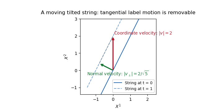
For the linear profile, the spatial string is the straight line $X^2=k{X}^1+kt$. It is tilted, and its coordinate intercept moves with speed $k$. This is also a uniformly moving straight string: the physical transverse velocity of a tilted string is the velocity normal to the line. With unit tangent $(1,k)/\sqrt{1+k^2}$ and coordinate velocity $(0,k)$, the normal speed isThus $k>1$ does not imply superluminal physical motion. Fixed-$\sigma$ labels have spacelike trajectories when $k>1$, but labels on a string can slide tangentially and are not identifiable material particles. Choosing $\dot{\sigma }=-k^2/(1+k^2)$ removes the tangential velocity and gives the subluminal velocity $(-k^2,k)/(1+k^2)$.

The induced worldsheet metric supplies a coordinate-invariant check:The string worldsheet remains Lorentzian for every finite $k$, including $k=1$ and $k>1$. Its constant energy density is $1+k^2$. This linear profile is a tilted boosted straight string, rather than a localized finite-energy wave.