Past exam of the mathematics course of the University of Cambridge / 2017 / iii / Paper 327 (Distribution Theory and Applications)

Use the Fourier transform convention $\hat{\phi }(\xi )=\int e^{-ix\cdot \xi }\phi (x)dx$ and $D_j=-i{\partial }_j$, so $\widehat{P(D)u}=P(\xi )\hat{u}$. All distribution pairings use complex bilinearity, and the formal transpose is $P(-D)$, without complex conjugation of the coefficients. If $D_j$ instead denotes ${\partial }_j$, the Fourier multiplier is $P(i\xi )$; the argument below is unchanged after this substitution.

For a nonempty compact convex set $K\subset {\mathbb{R}}^n$, let $H_K(\eta )={\sup }_{x\in K}x\cdot \eta$ be its support function. The Paley–Wiener–Schwartz theorem says that the Fourier transform is a bijection between distributions supported in $K$ and entire functions $F$ on ${\mathbb{C}}^n$ for whichfor some $C>0$ and nonnegative integer $N$. In particular, support in ${\overline{B}}_R$ is equivalent to the bound with $e^{R|\mathrm{Im}\zeta |}$. Convexity is essential in the precise support formulation: the support function of a set equals that of its convex hull.

Suppose first that $u$ is a compactly supported distribution with support in $K$. Define $F(\zeta )=⟨u,e^{-ix\cdot \zeta }⟩$, inserting any cutoff function equal to one near $K$ when viewing $u$ on test functions. A fixed cutoff and the finite order of a distribution estimate permit differentiation of the pairing in each complex variable, giving ${\partial }_{\zeta }^{\alpha }F=⟨u,(-ix{)}^{\alpha }{e}^{-ix\cdot \zeta }⟩$. The exponential function's power series converges with every required derivative on a fixed compact set; hence $F$ is an entire function. On real frequencies it agrees with the Fourier transform of a compactly supported distribution.

The exact exponential indicator needs a shrinking cutoff function, rather than one fixed outside $K$. Choose ${\chi }_{\epsilon }=1$ near $K$, with support in $K+B_{2\epsilon }$ and $\Vert {\partial }^{\alpha }{\chi }_{\epsilon }{\Vert }_{\infty }\le C_{\alpha }{\epsilon }^{-|\alpha |}$ for $0<\epsilon \le 1$. Such a cutoff is obtained by convolving the indicator of $K+B_{\epsilon }$ with a mollifier supported in $B_{\epsilon /2}$. On one fixed ball containing all these supports, the finite order of a distribution bound isThe Leibniz rule applied to $\theta ={\chi }_{\epsilon }{e}^{-ix\cdot \zeta }$ therefore givesTaking $\epsilon =(1+|\zeta |{)}^{-1}$ proves the required bound, with $N=2m$ and a fixed additional factor at most $e^2$.

Conversely, suppose $F$ is an entire function with the displayed bound. Its real restriction has polynomial growth, so its inverse Fourier transform defines a tempered distribution byRapid decay of the Schwartz function $\hat{\phi }$ makes this integral absolutely convergent and continuous in the Schwartz space topology.

To determine the support of a distribution, take a test function supported in a half-space $x\cdot \omega \ge H_K(\omega )+\delta$, where $|\omega |=1$ and $\delta >0$. The contour-shift proof of the Paley–Wiener–Schwartz theorem gives, for each $t\ge 0$,Here is the estimate that justifies both the shift and its limiting use. Since $\hat{\phi }(-\xi -it\omega )=\int e^{ix\cdot \xi }{e}^{-tx\cdot \omega }\phi (x)dx$, repeated integration by parts with $1-{\Delta }_x$ yieldsFor fixed $t$, the same estimate is uniform over the imaginary strip from $0$ to $t\omega$. Rotate coordinates so $\omega$ is the first coordinate direction, apply the Cauchy integral theorem on truncated rectangles, and let their real edges tend to infinity. If $2L>N+n$, the boundary integrals vanish and the horizontal integrals converge absolutely; thus the claimed shift is valid. Using $H_K(t\omega )=t{H}_K(\omega )$ now bounds the pairing bywhich tends to zero. A separating hyperplane exists at every point outside the compact convex set $K$. A finite partition of unity on the support of any exterior test function reduces it to such half-spaces, so $\mathrm{supp}u\subseteq K$. Fourier inversion gives uniqueness; the entire transform of this $u$ agrees with $F$ on ${\mathbb{R}}^n$ and hence everywhere, by applying the one-variable identity theorem successively in each coordinate. This completes both directions.

Now apply this theorem to compact support solvability for a constant-coefficient ordinary differential equation. If $P$ is a nonzero constant, its kernel is zero and $u=v/P$ is the unique solution. Otherwise writeThe solution space of $P(-D)\phi =0$ isIndeed these exponentials solve the equation, their initial derivative vectors have a nonzero Vandermonde determinant, and uniqueness for the order-$m$ ordinary differential equation makes them a basis. Pairing $P(D)u=v$ with any such solution proves necessity:

For sufficiency, choose $R$ with $\mathrm{supp}v\subseteq [-R,R]$ and let $V(\zeta )=⟨v,e^{-ix\zeta }⟩$. The assumed annihilation is precisely $V({\alpha }_j)=0$ for every $j$. Since all roots of a polynomial are simple, $U=V/P$ has removable singularities at every root and is an entire function. Outside one disk, $|P(\zeta )|\ge c(1+|\zeta |{)}^m$. Inside that disk, the extended $U$ is bounded. The polynomial division preservation of exponential type therefore givesThe Paley–Wiener–Schwartz theorem produces a compactly supported distribution $u$ with transform $U$, supported in the same interval. Then $\widehat{P(D)u}=PU=V$, so Fourier inversion gives $P(D)u=v$. ThusThe compactly supported solution is unique: $P\hat{u}=0$ forces the entire transform to vanish off the finitely many roots and hence everywhere. With repeated roots, the corresponding condition would also require derivatives $V^{(k)}(\alpha )=0$, or pairing with $x^k{e}^{-i\alpha x}$, up to one less than each multiplicity.

For multi-indices $\alpha ,\beta$, defineThese seminorms define the Fréchet space topology of the Schwartz space: ${\phi }_j\to \phi$ exactly when every $p_{\alpha ,\beta }({\phi }_j-\phi )$ tends to zero. An equivalent increasing family isA tempered distribution is a continuous linear functional on this space. Equivalently, $|⟨T,\phi ⟩|\le C{q}_m(\phi )$ for some $C,m$. The usual weak convergence of tempered distributions means $⟨T_j,\phi ⟩\to ⟨T,\phi ⟩$ for every fixed Schwartz function. The strong dual topology instead requires uniform convergence on every subset of the Schwartz space that is a bounded set in a topological vector space; the Fourier maps below are continuous in both topologies.

Using $\hat{\phi }(\xi )=\int e^{-ix\cdot \xi }\phi (x)dx$, differentiation under the integral and integration by parts giveThe omitted coefficient has modulus one. By the Leibniz rule, every integrand is a finite sum of a polynomial times a derivative of $\phi$. Inserting the integrable weight $(1+|x|{)}^{-n-1}$ bounds its L1 norm by finitely many Schwartz space seminorms. In particular $q_m(\hat{\phi })\le C_m{q}_{m+n+1}(\phi )$. Thus the Fourier transform maps $\mathcal{S}$ continuously into itself.

For completeness, the Fourier inversion theorem follows here by Gaussian regularization. The inverse transform of $e^{-t|\xi {|}^2}$ is $g_t(x)=(4\pi t{)}^{-n/2}{e}^{-|x{|}^2/(4t)}$. The Fourier transform of a Gaussian and Fubini's theorem showAs $t\downarrow 0$, the right side tends to $\phi (x)$ by the approximate identity property, while the left side tends to the undamped inverse integral by dominated convergence theorem, since $\hat{\phi }\in L^1$. HenceThe inverse is $(2\pi {)}^{-n}$ times reflection composed with the continuous Fourier transform, and is therefore continuous on the Schwartz space. This proves a continuous linear isomorphism with continuous inverse.

Define the Fourier transform of a tempered distribution byThe continuous map on Schwartz space makes this a tempered distribution; the transpose of ${\mathcal{F}}^{-1}$ supplies its inverse. Pointwise convergence of pairings proves weak continuity. For the strong dual topology, the transform of a bounded set of Schwartz functions is bounded, so uniform convergence of pairings on bounded sets proves continuity of both Fourier maps there too.

Now let $R\in SO(n)$ be a rotation matrix in the special orthogonal group and write ${\rho }_{R}T=T\circ R$. A change of variables with unit Jacobian givesThe rotation equivariance of the Fourier transform on tempered distributions follows by duality:Therefore $\widehat{{\rho }_{R}T}={\rho }_R\hat{T}$. Applying this identity and the inverse Fourier transform gives the two directions:This is precisely preservation of radial tempered distributions. For $n>1$, $SO(n)$ acts transitively on spheres, so an invariant smooth function is an ordinary radial function.

The multiplication of a distribution by a smooth function is $⟨\psi T,\phi ⟩=⟨T,\psi \phi ⟩$. If $\psi$ is a Schwartz function, the Leibniz rule shows that $\phi \mapsto \psi \phi$ is a continuous map $\mathcal{S}\to \mathcal{S}$, so $\psi T$ is a tempered distribution. When both $\psi$ and $T$ are radial, $\psi \circ R^t=\psi$, andThus Multiplication by a radial Schwartz function preserves radial tempered distributions.

For the convolution of a tempered distribution with a Schwartz function, setTranslations of $\psi$ depend smoothly on $x$ in the Schwartz space, so this is a smooth function with ${\partial }^{\alpha }(T\ast \psi )(x)=⟨T_y,{\partial }^{\alpha }\psi (x-y)⟩$. The bound for $T$ by finitely many seminorms, together with $1+|y|\le (1+|x|)(1+|x-y|)$, provesThus the function also defines a tempered distribution. For a radial function $\psi$, put $g_x(y)=\psi (x-y)$. Then $\psi (Rx-y)=\psi (x-R^{t}y)=g_x(R^{t}y)$, soHence Convolution with a radial Schwartz function preserves radial tempered distributions.

Smoothing alone need not give a Schwartz function: for the constant tempered distribution $T=1$ and a Schwartz function with integral one, $T\ast \psi =1$. The radial Schwartz approximation of tempered distributions therefore combines smoothing with a large-radius cutoff. Choose a nonnegative radial mollifier $\rho \in C_c^{\infty }$, supported in the unit ball with integral one, and a radial cutoff function $\chi \in C_c^{\infty }$ equal to one on the unit ball. PutEach $f_j$ is a smooth function of compact support, hence a Schwartz function, and the two invariance calculations above make it radial.

It remains to prove convergence, including the simultaneous changes of both scales. With $\check{\rho }(x)=\rho (-x)$, the distributional convolution pairing isFor every fixed $m$, the Leibniz rule, rapid decay outside the radius-$j$ ball, and the chain rule for $\chi (x/j)$ giveConvolution by ${\check{\rho }}_{\epsilon }$ is uniformly bounded in $q_m$ for $0<\epsilon \le 1$, because its shifts have size at most one. The mean value theorem applied to $\phi (x-y)-\phi (x)$ similarly givesSplitting the error into the convolved cutoff error and the approximate identity error provesIf $|⟨T,\theta ⟩|\le C{q}_m(\theta )$, this yieldsConsequentlyweakly, and even in the strong dual topology, since $q_{m+1}$ is uniformly bounded on every subset of the Schwartz space that is a bounded set in a topological vector space. No assertion that $T\ast {\rho }_{1/j}$ itself is rapidly decreasing is needed.

Again use $D_j=-i{\partial }_j$ and distribution dual pairings with complex bilinearity. The Malgrange–Ehrenpreis theorem asserts that every nonzero constant-coefficient differential operator defined by a polynomial has a fundamental solution of a linear differential operator:If $P=a\ne 0$ is constant, take $E={\delta }_0/a$. For positive degree $m$, write $P_m$ for the highest homogeneous part. A nonzero polynomial cannot vanish on all of ${\mathbb{R}}^n$, so choose a real unit vector $e$ with $P_m(e)\ne 0$. A change of coordinates by an orthogonal matrix makes it the last coordinate direction. In these coordinates,Crucially the leading coefficient $a$ is constant and never vanishes as ${\xi }^{\prime }\in {\mathbb{R}}^{n-1}$ varies.

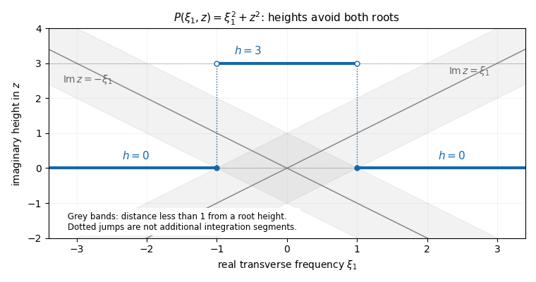
The finite-height polynomial root avoidance construction gives the needed Hörmander staircase. Set $h_{\ell }=3\ell$ for $0\le \ell \le m$. For each fixed ${\xi }^{\prime }$, the fundamental theorem of algebra supplies $m$ roots $z_1,\dots ,z_m$, with multiplicity. A root's imaginary part can be within distance strictly less than one of at most one candidate height, since those heights are separated by three. The pigeonhole principle therefore leaves at least one height with $|h_{\ell }-\mathrm{Im}{z}_j|\ge 1$ for all roots. At that height, for every real $s$,No continuous labelling of the roots is required. To select the heights measurably, defineEach $B_{\ell }$ is closed, since the coefficients are continuous in ${\xi }^{\prime }$. Continuity in $s$ makes the rational test equivalent to the bound for all $s\in \mathbb{R}$. The $A_{\ell }$ are therefore disjoint Borel sets covering ${\mathbb{R}}^{n-1}$. The union of horizontal fibresis a Hörmander staircase, with bounded imaginary height and a uniform nonzero denominator. For $n=1$, the transverse space has one point, and this is simply the choice of one horizontal line.

For example, $P({\xi }_1,z)={\xi }_1^2+z^2$ has roots $z=\pm i{\xi }_1$. One may select $h=0$ for $|{\xi }_1|\ge 1$, and $h=3$ for $|{\xi }_1|<1$. Then the first region has $|P|\ge 1$, while in the second each root is at least two units from the chosen height. The figure shows the height projection of these horizontal fibres, rather than additional connecting contours.

Define a linear functional on test functions byTo establish that this is a distribution, fix a compact set containing the support of $\phi$, inside a radius-$R$ ball. The Fourier decay in a bounded complex strip estimate follows by applying $(1-\Delta {)}^L$ to $e^{-h_{\ell }{x}_n}\phi (x)$:The finite bound on the heights absorbs all exponential factors and powers of $h_{\ell }$ into $C_{R,L}$. Taking $2L>n$ and using $|P|\ge |a|$ proves absolute convergence and the required finite-order continuity on each fixed support set. Hence $E\in {\mathcal{D}}^{\prime }$.

Now the formal transpose identity and the Fourier derivative identity giveThe polynomial denominator cancels in the pairing for $P(D)E$. For each fixed real ${\xi }^{\prime }$, the remaining function of $z$ is entire and rapidly decreasing in its real part throughout $0\le \mathrm{Im}z\le 3m$. The Cauchy integral theorem therefore allows each horizontal fibre to be shifted to the real axis; its truncated vertical end integrals tend to zero. Absolute convergence justifies Fubini's theorem and the finite sum over the measurable partition. ThusThe last equality is Fourier inversion. Transforming back from the orthogonal coordinates preserves ${\delta }_0$ and gives the required fundamental solution of a linear differential operator for the original operator. The staircase is allowed to jump: after cancellation the shift is performed on each one-dimensional fibre, so no assertion that $\Sigma$ is a smooth contour is used. This construction proves a distributional fundamental solution, without claiming a tempered-growth estimate.

For $f\in \mathcal{D}({\mathbb{R}}^n)$, use the smoothing convolution with a test functionIndeed $u_0(x)=⟨E_y,f(x-y)⟩$ is a smooth function, with ${\partial }^{\alpha }{u}_0(x)=⟨E_y,{\partial }^{\alpha }f(x-y)⟩$. On each compact set of $x$ values, all translated test functions have supports in one fixed compact set, so differentiation is justified by the continuity of the distribution. Compact support of $f$ makes the convolution well defined even when $E$ is not tempered. It does not imply compact support of $u_0$.

Finally the affine solution space of a linear equation isIf every homogeneous solution is represented by a smooth function, so is every $u=u_0+v$. Conversely, if every solution for this fixed $f$ is represented by a smooth function, then for any homogeneous solution $v$, the solution $u_0+v$ is smooth, and subtracting the smooth $u_0$ shows that $v$ is smooth. Hence All inhomogeneous solutions are smooth functions exactly when all homogeneous solutions are smooth functions. This is a global statement on ${\mathbb{R}}^n$ for the stated data; no additional local regularity theorem is being assumed.