Adaptive optics corrects rapidly changing atmospheric wavefront errors to improve angular resolution and image concentration. A wavefront sensor estimates those errors and a feedback controller commands a deformable mirror to oppose them, aiming toward the diffraction limit of a telescope rather than the uncorrected astronomical seeing limit.
The main optical path is telescope to deformable mirror to beam splitter to science camera. The splitter also directs reference light to a wavefront sensor; a controller reconstructs the wavefront error and feeds mirror commands back to the deformable mirror. The mirror is normally conjugate to a pupil so its actuators address the corresponding pupil phase. A separate steering mirror can handle overall image motion.
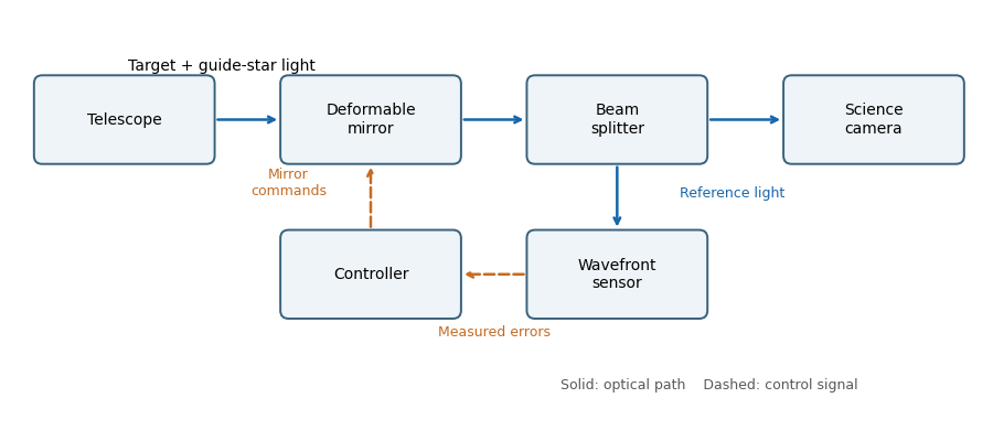
An adaptive-optics feedback loop
. Solid arrows show optical paths. The wavefront sensor observes the corrected reference beam; dashed arrows return measured errors and actuator commands through the controller. The science beam shares the deformable mirror. Details.
The Strehl ratio isusing the same total flux, pupil, and wavelength for both images. A value near one means that little light has been redistributed from the ideal central peak by wavefront errors. For small residual phase variance , the Maréchal approximation is , with for the residual optical-path root mean square error.
Adaptive-optics sky coverage is limited by the need for a guide star bright enough to measure the wavefront error on the atmospheric evolution time. A faint guide gives noisy measurements; a guide too far from the target samples a different turbulent column. That angular mismatch is anisoplanatism, with useful separation characterized by the isoplanatic angle. Thus a conventional single-guide system cannot provide equally good correction at every target position.
A laser guide star supplies an artificial bright reference and improves coverage. However, its finite-distance beam does not sample the full stellar turbulence column, and conventional laser systems need a natural reference for absolute image motion. The required reference brightness, angular separation, and desired correction quality therefore still constrain observations.
Astronomical seeing is the atmospheric angular blurring of a point-source image, usually reported in arcseconds. Operationally it is commonly characterized by the full width at half maximum of a long-exposure stellar point spread function. The full observed width can also contain telescope and instrumental contributions; the atmospheric seeing is the turbulence contribution.
For a large aperture in the standard turbulence model, astronomical seeing is approximately radians, with Fried parameter . Maintaining comparable correction requires a deformable mirror actuator pitch of order , so the number of actuators across a diameter is proportional to and the total illuminated actuator count is proportional to . ThereforeLonger wavelengths require fewer actuators and have slightly smaller uncorrected atmospheric angular blur, even though the telescope's diffraction-limited resolution scale increases with wavelength.
For the unnormalized Zernike polynomial with , the three radial terms areSince ,Along a central chord with signed coordinate , replace by . The profile is even, equals one at the center and both edges, and has minima at . This Zernike spherical mode corresponds to primary spherical aberration, balanced by defocus and piston terms rather than simply the raw quartic Seidel term.
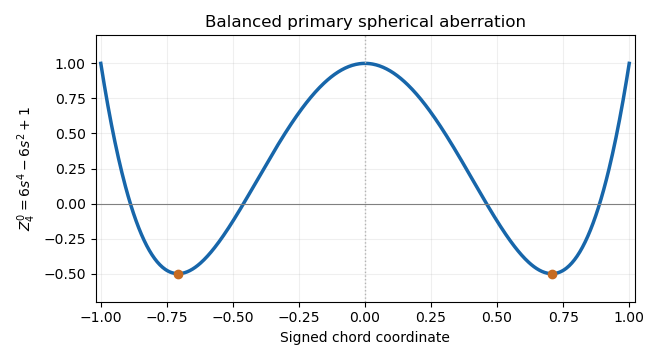
The unnormalized Zernike spherical mode on a central chord
. The even quartic has central and edge values one and two minima of minus one half. Its lower-order terms remove its projections onto piston and defocus. Details.
The projected actuator pitch is in the question's sampling convention. A sinusoidal wavefront error needs at least two samples per spatial period, by the Nyquist–Shannon sampling theorem. Thus the shortest limiting correctable scale at the primary isThe Nyquist spatial frequency is cycles per unit length. Exactly at that limiting frequency some phases are poorly sampled; actual deformable mirror performance also depends on actuator influence functions, so this is an ideal bandwidth limit.
Count independent sinusoidal ripples by their spatial Fourier series indices. A mode with cycles across has , so the given half-wave index is . The Nyquist spatial frequency permits . In two dimensions, a circular cutoff therefore contains approximately integer wavevectors.
For a real wavefront error, the wavevectors and describe the same ripple with conjugate coefficients, so count each pair once. The continuum mode-counting approximation givesThis counts one ripple with amplitude and phase per conjugate pair, not one real coefficient. Exact finite-grid counts are integers and have boundary corrections; the formula is the circular area estimate implicit in the question, with piston excluded.
The supplied speckle contrast of a sinusoidal wavefront error gives . Each sinusoid has root mean square error . For orthogonal modes, or for uncorrelated phases so that cross terms average to zero, the total mean square adds:Therefore the assumed equal-contrast modal model givesIf the individual contrasts are not equal, the corresponding formula is . The error here is optical-path wavefront error; for a near-normal reflecting mirror, physical surface error is half the optical-path error.
A wavefront error ripple of period generates a pair of speckles at angular displacement . Combining this with gives the deformable-mirror control radius along an actuator row or column:A square actuator lattice has a square ideal frequency region: . Its full width is , approximately diffraction-limited resolution elements per side, or in area. The circular subset within the row-direction radius contains approximately such elements. The primary aperture shapes each speckle's point spread function; it does not turn the square sampling limit into a circular one.
Articles by others on the same topic
There are currently no matching articles.