The bright peaks occur when contributions from adjacent grooves have equal phase modulo , so all illuminated grooves contribute by constructive interference. Use the reflection-grating convention shown below: and are positive angles of the incident and outgoing ray lines on the same side of the normal. The incoming and outgoing path differences between neighboring grooves are and , respectively. Hence the grating equation isThe integer labels the diffraction order. With a different signed-angle convention, the same physical condition contains a difference of sines.
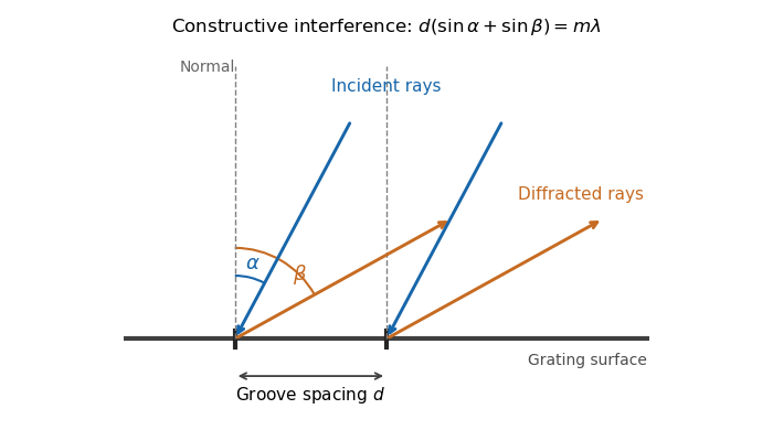
Reflection-grating angle convention
. The incident ray and selected outgoing ray are both drawn on the positive side of the surface normal. Adjacent groove spacing contributes the sum of their two projected path differences. Details.
At fixed incidence angle, differentiation of the grating equation gives . Near the camera axis, the focal-plane displacement is , so the local grating dispersion isIt has units of distance per unit wavelength. If the camera axis is at and the flat focal-plane coordinate is retained exactly as , thenThe boxed expression is the local value at the optical axis.
In the simple slit-image approximation, the projected slit width is . Equating this width to the separation of barely resolved features, using the grating dispersion, givesThis recovers the stated spectral resolving power under the assumption that the grating has unit anamorphic magnification.
For arbitrary distinct and , the anamorphic magnification of a grating must be included. At fixed wavelength, the grating equation gives , so the slit image instead has width . Thus the general slit-limited resolving power of a grating isThe two expressions agree in the Littrow configuration, . Without that condition or the unit-magnification approximation, the quoted expression is not the general slit-limited result. Finite grating size, detector sampling, and optical aberrations can lower the actual resolution further.
The echellogram contains nearly parallel traces, one for each diffraction order. Choose the main echelle grating dispersion to increase wavelength toward the right and the cross-disperser to increase wavelength upward. At a fixed horizontal coordinate, order has a shorter wavelength than order , so it lies below order in this convention.
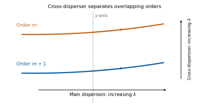
Adjacent orders in a cross-dispersed echellogram
. Order m+1 is bluer than order m at the same main-dispersion coordinate. Within either order, wavelength increases along the trace to the right; the chosen cross-dispersion orientation puts longer wavelengths higher on the detector. Details.
Let be the central camera direction. The grating equation fixesThe usual adjacent-order free spectral range of an echelle grating is thereforeThe constant has dimensions of length and is the path difference between adjacent grooves for light directed along the camera axis; it is also the fixed product . Near the Littrow configuration, . The detector width corresponding to this interval is approximately , with grating dispersion .
There is a convention issue in reading the question literally. Adjacent order-center separation is exactly the expression above. A partition assigning each wavelength to whichever order lands closest to the vertical axis has boundaries halfway in detector displacement, not at adjacent order centers. In the small-angle detector approximation its boundaries for order are and , giving width . Both conventions give for high orders, but their exact finite- widths differ. The quoted expression is the conventional adjacent-order spacing.
The magnitude zero point is defined by the reference response . With zero magnitude assigned to that reference, the apparent magnitude isThe two responses must use the same photometric passband and instrumental weighting. If the reference has assigned magnitude instead, add to the right-hand side.
The traditional infrared photometric bands extending the optical photometric system into this range are approximatelyTheir photometric passbands lie mainly in atmospheric windows between strong molecular absorption bands. This makes ground-based observations practical. The exact centers depend on the system: is near , and shortened and bands reduce unwanted background or absorption. At the longest wavelengths, atmospheric and instrumental thermal radiation make sky brightness especially important. A modern band near is an additional choice, rather than one of the traditional extensions.
For identical luminosities in a uniform Euclidean distribution, the inverse-square law gives flux , while the number of sources within distance is proportional to . Therefore ten times as many objects require and . Applying the definition of apparent magnitude givesThis is the Euclidean magnitude-limited source count relation. It assumes no extinction, spatial variation of density, or cosmological change in the flux-distance relation.
Atmospheric extinction changes the amplitude of the incoming light through absorption and scattering. Its wavelength dependence alters the measured optical spectrum and colors; clouds and aerosols introduce additional time dependence. Scattered moonlight and atmospheric emission increase sky brightness.
Atmospheric refraction changes the apparent position of the source. Its wavelength dependence, atmospheric dispersion, spreads a broadband image toward the zenith. The mean refractive index gradient therefore affects direction even in the absence of small-scale turbulence.
Atmospheric turbulence produces rapidly varying optical path lengths, distorting the phase and curvature of a nominally plane wavefront. Different pupil regions acquire different phase delays, producing astronomical seeing, image motion, and short-exposure speckle patterns. Different lines of sight sample different fluctuations, giving anisoplanatism.
Propagation through the fluctuating medium also changes the intensity through atmospheric scintillation, the familiar twinkling of stars. A phase-only adaptive optics correction can reduce atmospheric phase errors but does not remove absorption, all scintillation, or the atmospheric emission background.
Adaptive optics corrects rapidly changing atmospheric wavefront errors to improve angular resolution and image concentration. A wavefront sensor estimates those errors and a feedback controller commands a deformable mirror to oppose them, aiming toward the diffraction limit of a telescope rather than the uncorrected astronomical seeing limit.
The main optical path is telescope to deformable mirror to beam splitter to science camera. The splitter also directs reference light to a wavefront sensor; a controller reconstructs the wavefront error and feeds mirror commands back to the deformable mirror. The mirror is normally conjugate to a pupil so its actuators address the corresponding pupil phase. A separate steering mirror can handle overall image motion.
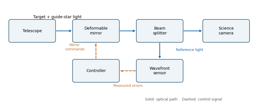
An adaptive-optics feedback loop
. Solid arrows show optical paths. The wavefront sensor observes the corrected reference beam; dashed arrows return measured errors and actuator commands through the controller. The science beam shares the deformable mirror. Details.
The Strehl ratio isusing the same total flux, pupil, and wavelength for both images. A value near one means that little light has been redistributed from the ideal central peak by wavefront errors. For small residual phase variance , the Maréchal approximation is , with for the residual optical-path root mean square error.
Adaptive-optics sky coverage is limited by the need for a guide star bright enough to measure the wavefront error on the atmospheric evolution time. A faint guide gives noisy measurements; a guide too far from the target samples a different turbulent column. That angular mismatch is anisoplanatism, with useful separation characterized by the isoplanatic angle. Thus a conventional single-guide system cannot provide equally good correction at every target position.
A laser guide star supplies an artificial bright reference and improves coverage. However, its finite-distance beam does not sample the full stellar turbulence column, and conventional laser systems need a natural reference for absolute image motion. The required reference brightness, angular separation, and desired correction quality therefore still constrain observations.
Astronomical seeing is the atmospheric angular blurring of a point-source image, usually reported in arcseconds. Operationally it is commonly characterized by the full width at half maximum of a long-exposure stellar point spread function. The full observed width can also contain telescope and instrumental contributions; the atmospheric seeing is the turbulence contribution.
For a large aperture in the standard turbulence model, astronomical seeing is approximately radians, with Fried parameter . Maintaining comparable correction requires a deformable mirror actuator pitch of order , so the number of actuators across a diameter is proportional to and the total illuminated actuator count is proportional to . ThereforeLonger wavelengths require fewer actuators and have slightly smaller uncorrected atmospheric angular blur, even though the telescope's diffraction-limited resolution scale increases with wavelength.
For the unnormalized Zernike polynomial with , the three radial terms areSince ,Along a central chord with signed coordinate , replace by . The profile is even, equals one at the center and both edges, and has minima at . This Zernike spherical mode corresponds to primary spherical aberration, balanced by defocus and piston terms rather than simply the raw quartic Seidel term.
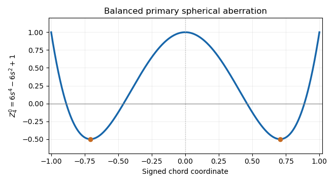
The unnormalized Zernike spherical mode on a central chord
. The even quartic has central and edge values one and two minima of minus one half. Its lower-order terms remove its projections onto piston and defocus. Details.
The projected actuator pitch is in the question's sampling convention. A sinusoidal wavefront error needs at least two samples per spatial period, by the Nyquist–Shannon sampling theorem. Thus the shortest limiting correctable scale at the primary isThe Nyquist spatial frequency is cycles per unit length. Exactly at that limiting frequency some phases are poorly sampled; actual deformable mirror performance also depends on actuator influence functions, so this is an ideal bandwidth limit.
Count independent sinusoidal ripples by their spatial Fourier series indices. A mode with cycles across has , so the given half-wave index is . The Nyquist spatial frequency permits . In two dimensions, a circular cutoff therefore contains approximately integer wavevectors.
For a real wavefront error, the wavevectors and describe the same ripple with conjugate coefficients, so count each pair once. The continuum mode-counting approximation givesThis counts one ripple with amplitude and phase per conjugate pair, not one real coefficient. Exact finite-grid counts are integers and have boundary corrections; the formula is the circular area estimate implicit in the question, with piston excluded.
The supplied speckle contrast of a sinusoidal wavefront error gives . Each sinusoid has root mean square error . For orthogonal modes, or for uncorrelated phases so that cross terms average to zero, the total mean square adds:Therefore the assumed equal-contrast modal model givesIf the individual contrasts are not equal, the corresponding formula is . The error here is optical-path wavefront error; for a near-normal reflecting mirror, physical surface error is half the optical-path error.
A wavefront error ripple of period generates a pair of speckles at angular displacement . Combining this with gives the deformable-mirror control radius along an actuator row or column:A square actuator lattice has a square ideal frequency region: . Its full width is , approximately diffraction-limited resolution elements per side, or in area. The circular subset within the row-direction radius contains approximately such elements. The primary aperture shapes each speckle's point spread function; it does not turn the square sampling limit into a circular one.
This full square describes phase-error control. Simultaneous amplitude and phase correction with a single pupil-plane deformable mirror generally requires restricting the dark region to a half-plane; it is a different constraint from the sampling bandwidth.
Let and be the real object and image distances from the thin lens. The object-screen separation gives , and the thin lens equation gives . Thus the two lens positions solveTheir separation is , soThis is the Bessel lens displacement method for measuring focal length. It uses the screen-object separation and the displacement between two sharp-image settings, reducing the need to locate the lens's effective optical center. It assumes the thin-lens or corresponding principal-plane approximation; is what provides two distinct real-image settings.
For thin lenses in contact, optical powers add. At the two reference wavelengths, the lensmaker's equation gives total powerAn achromatic lens has . Subtracting and solving for the curvature-factor ratio yieldsOpposite curvature-weighted powers compensate the two materials' optical dispersion.
At the intermediate reference wavelength, the lensmaker's equation gives . Therefore the curvature-factor ratio from the previous part impliesand henceThe last equality uses the Abbe number definition and expresses the achromatic doublet power balance in terms of component focal lengths.
Write and . The achromatic doublet power balance isSolving these two linear equations gives and . Taking reciprocals gives the required focal lengths:The design requires distinct Abbe numbers; identical relative dispersion cannot yield a nonzero total achromatic power from this two-element thin model.
is the Abbe number, a measure of inverse relative optical dispersion. Ordinary crown glasses have comparatively large and lower refractive index, while ordinary flint glasses have smaller and often higher index. The Abbe diagram below spans typical optical-glass values; the shaded family ranges are schematic, and the marked examples are catalogue data. Modern glass compositions broaden and overlap the simple crown/flint picture.
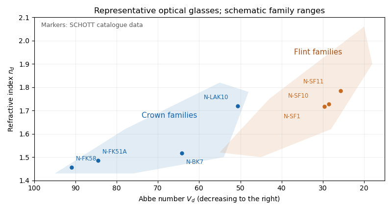

For a positive doublet with , the preceding formulas require and : a converging crown glass element and a diverging flint glass element. Their dispersion corrections cancel, while their net optical power is positive. A small difference in Abbe numbers requires large opposing component powers, which makes the design harder to correct for other optical aberrations.
Let the two internal angles be and , since the optical prism geometry gives . By Snell's law, the corresponding external angles are and , where . The deviation isOn the transmitted branch with and ,Thus is strictly increasing. The stationary condition forces , and the positive second derivative makes this the unique minimum deviation. ConsequentlyThe argument assumes a transmitted ray is possible; the symmetric internal angles must lie below the critical angle.
The reversibility of an optical ray interchanges entry and exit while preserving the total deviation. Away from the turning point, a ray and its reversed configuration give the same deviation with the entry and exit angles exchanged. At minimum deviation the two configurations merge: the path is symmetric and the entry and exit angles are equal.
Physically, distributing the refraction symmetrically between the two faces avoids making one face contribute disproportionately large bending. The strict convexity established in the preceding part proves that this stationary symmetric configuration is the minimum, rather than merely following from reversibility alone.
At minimum deviation, and . Substituting in Snell's law givesFor a known prism apex angle, measuring the minimum deviation with monochromatic light determines its refractive index. Repeating the measurement at several wavelengths measures optical dispersion. If the surrounding medium is not air, the measured ratio is relative to that medium's refractive index.
The two standard designs are multi-slit spectrographs and fiber-fed spectrographs. Both select many astronomical targets simultaneously and arrange their light so the resulting optical spectra remain distinguishable on the detector.
A multi-slit spectrograph uses a focal-plane mask containing slitlets at the target positions, or movable slitlets placed there. Each transmits its target and nearby sky into the collimator; a diffraction grating or other disperser produces a separate optical spectrum on the detector. The layout must avoid overlap between spectra, and the length of a slit allows local sampling of sky brightness and sometimes spatial information within the target.
A fiber-fed spectrograph places optical fibers at target positions in the telescope focal plane. The fibers carry the selected light to a spectrograph and their outputs are lined up as a pseudo-slit. The spectrograph can be mechanically stable and separate from the telescope's focal plane. Additional fibers aimed at blank sky provide a simultaneous estimate of sky brightness; fiber positioning, coupling losses, transmission, and focal-ratio degradation must be accounted for.
For field of view, fiber-fed spectrographs commonly cover wider sky areas: fibers can pick targets across a broad focal plane while feeding a compact spectrograph with a fixed output slit. A multi-slit spectrograph must image its field through the spectrograph optics, and spectra must fit on the detector without overlap, which restricts both field and target layout.
For spectral resolution, fibers can feed an optimized, stable high-dispersion instrument, including an echelle grating. The fiber image acts as its entrance width. In a multi-slit spectrograph, slit width and dispersion similarly determine the spectral resolving power. Neither feed type alone imposes a universal resolution ranking: narrower fibers or slits improve resolution at the cost of losing source light, and both can be designed for high or low resolution.
For faintness limit, slit masks often have an advantage for individual faint objects because they avoid fiber coupling and transmission losses, permit a slit width matched to astronomical seeing, and sample local sky along the slit. Fibers can admit more sky through a fixed circular aperture and require sky subtraction from separate locations; focal-ratio degradation can also reduce throughput. The actual limit depends on throughput, aperture size, background stability, and detector noise through the signal-to-noise ratio in photon counting. Well-designed fiber instruments can nevertheless be very efficient for wide-field surveys, so the comparison is conditional on the optical design and observing conditions.
Articles by others on the same topic
There are currently no matching articles.