Past exam of the mathematics course of the year 1 of the natural sciences course of the University of Cambridge / 2021 / Paper 2 / 12

At a differentiable interior stationary point, all first-order changes of the scalar field vanish. In particular, the directional derivative along each coordinate axis vanishes, so $f_x=f_y=0$ and hence $\nabla f=0$. Equivalently, the first-order differential $df=\nabla f\cdot d\mathbf{r}$ vanishes for every displacement. A differentiable interior maximum or minimum must satisfy this condition; a stationary point need not be an extremum.

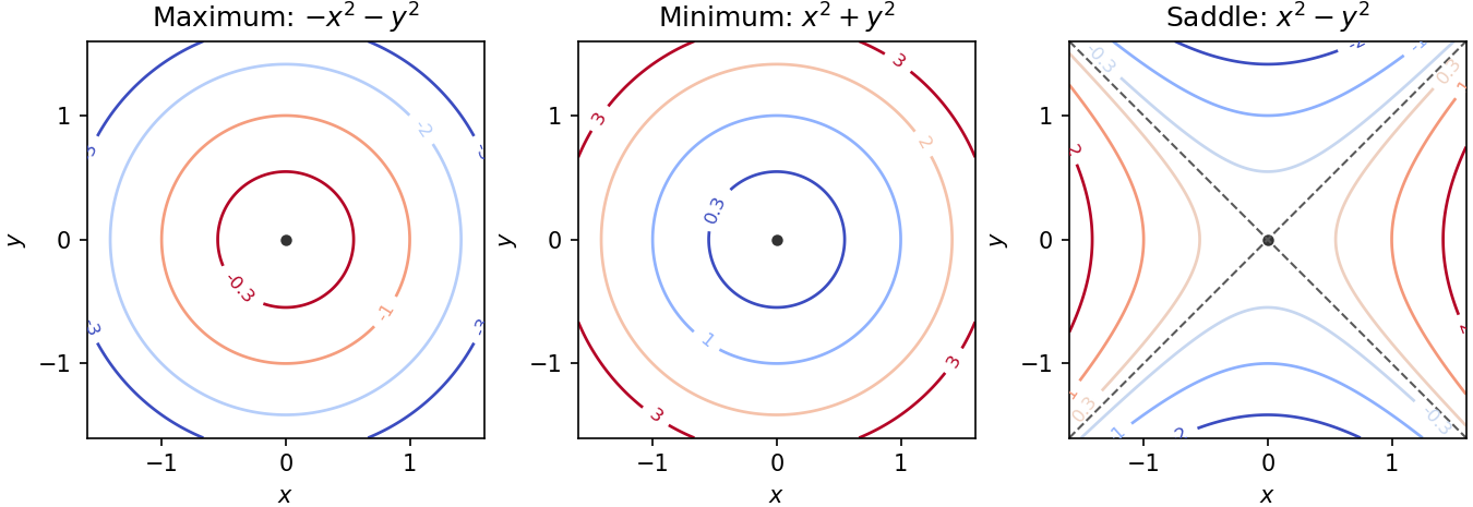
The standard nondegenerate local contour plot models are $-x^2-y^2$ for a maximum, $x^2+y^2$ for a minimum, and $x^2-y^2$ for a saddle point of a scalar function. Near a maximum, nested contours have lower values farther from the centre; near a minimum they have higher values. Near a saddle, hyperbolas occur on opposite sides of the critical level, whose contour has two intersecting tangent directions. More general nondegenerate quadratic forms deform these circles into ellipses; degenerate stationary points can have more complicated contours.

Set $D=1+x^2+y^2>0$. The quotient rule gives the partial derivativesSince $1+y+y^2=(y+1/2{)}^2+3/4>0$, the first equation $f_x=0$ forces $x=0$. The second then reduces to $1-y^2=0$. Thus the only stationary points and their field values areNo division by a potentially vanishing factor of $y$ was used, so no stationary points have been discarded.

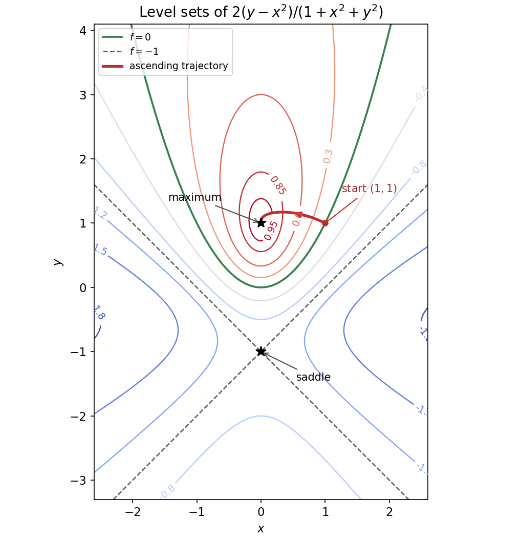
The level set $f=c$ can be rearranged, without changing its domain, asThe requested special contours are thereforeThe first is a parabola, the second a single point, and the last two intersecting straight lines. Moreoverwith equality only at $(0,1)$. Hence $(0,1)$ is a strict global maximum. At $(0,-1)$ the crossing critical contour separates sectors with values above and below $-1$, so it is a saddle point of a scalar function.

As a Hessian matrix check, $H_f(0,1)=\mathrm{diag}(-3,-1)$ is negative definite, while $H_f(0,-1)=\mathrm{diag}(-1,1)$ is indefinite. There is no stationary minimum.

For $c\ne 0$, completing the square gives the conic sectionThe possible levels follow fromFor $0<c<1$, the contours are ellipses centred at $(0,1/c)$, shrinking to the maximum as $c\uparrow 1$. The zero contour is the parabola from part (c). For $-1<c<0$, the contours are vertical-opening hyperbolas. At $c=-1$ they degenerate into the intersecting straight lines, and for $-2<c<-1$ they are horizontal-opening hyperbolas. These descriptions specify the remaining contour families and their symmetry about the $y$ axis. The lower bound $-2$ is approached as $|x|\to \infty$ at fixed $y$ but is never attained.

Use the gradient flow of $-f$, namely $\dot{\mathbf{r}}=\nabla f$; any positive change of speed leaves the same trajectory. At the starting point,so the path initially points up and left, with slope $dy/dx=-1/2$. At every regular point it crosses the level sets orthogonally, because the gradient is normal to the contours. Along it,until a stationary point is approached.

The red curve in the plot first rises above $y=1$, then bends down towards the maximum $(0,1)$. It stays on the side $x>0$ and approaches the maximum without crossing it in finite gradient-flow time. Indeed $\dot{x}=-4x(1+y+y^2)/D^2$ preserves the sign of $x$, and the critical level increases from its starting value $0$ towards $1$. The requested curve is an ascending trajectory, not a contour or a straight segment joining the initial and final points.