The two orthogonal directions and are preserved by this symmetric matrix. Direct multiplication, using the hyperbolic function identities , gives the eigenvalue–eigenvector pairsEach eigenvector can be multiplied by any nonzero scalar. For these give the two one-dimensional eigenspaces. When , the matrix is the identity: the only eigenvalue is , with multiplicity two, and every nonzero vector is an eigenvector.
The boundary order fixes the orientation. Two edges issuing from are and . Their cross product gives the oriented vector area:Its norm is , the ordinary rectangle area. The sign agrees with traversing by the right-hand orientation rule.
For this first-order linear differential equation, the integrating factor is . Thusand the general solution is
For , the change of variables reduces the integral to the given Gaussian integral:For , the integrand is an integrable odd function, so its contributions from the two half-lines cancel:The condition ensures convergence in both cases.
Complete the square in the velocity variable:Since , the final term is nonpositive and vanishes at exactly one velocity. ThereforeThis is the Legendre transform in mechanics that constructs the Hamiltonian mechanics energy from the kinetic-minus-potential Lagrangian.
Normalization of the probability mass function and the geometric series giveThe tail is another geometric series:
Substitute into the geometric series, without taking any derivatives:Thus the coefficient of in the Taylor series is when is even and zero when is odd. If nonzero terms are numbered from one, the th term is .
The chain rule givesFor this to vanish for every differentiable , its coefficient must be zero:The resulting is a profile transported to the right at unit speed by the transport equation.
On the disc , the upward normal selects only the third component, which equals . Hence the surface integral is the area of the unit disk:
The cross product of the direction vectors is . It is nonzero, so a common perpendicular direction exists. Projecting onto its unit vector gives the distance between skew lines:ThusThe numerator is a scalar triple product; movement along either line does not change this perpendicular projection.
Use only the dot product to minimize the squared Euclidean distance from the origin:Completing the square givesThe square is minimized at , yieldingGeometrically this subtracts the squared length of the orthogonal projection parallel to the line. At the minimizing point, , as required for perpendicular distance.
Here , and . ThereforeThe closest point has parameter and position , whose norm gives the same result.
For a point , the magnitude of is the area of a parallelogram. Dividing by its base length gives the perpendicular Euclidean distance to the first line. Explicitly,HenceThis use of the cross product removes any component parallel to the first line automatically.
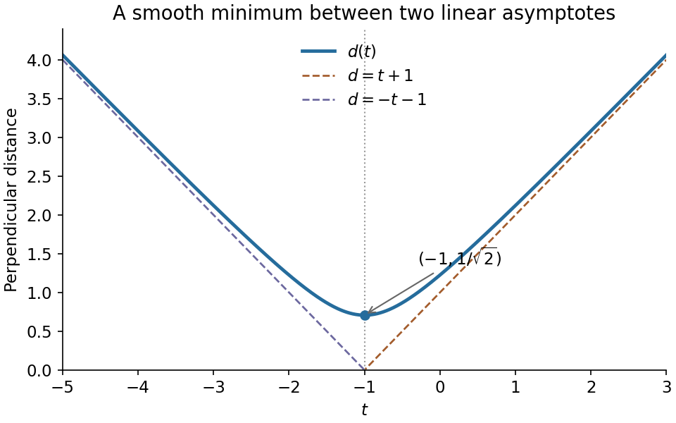
The graph is the upper branch of the hyperbola . It is symmetric about , positive everywhere, and has its lowest point at . Its derivatives areso it is strictly convex. Sinceits two oblique asymptotes are

The square is minimized when its first term vanishes. ThereforeThis agrees with the distance between skew lines found in part (b). The corresponding parameter on the first line is its orthogonal projection valueThe closest pair is and ; their connecting vector is perpendicular to both direction vectors.
At a differentiable interior stationary point, all first-order changes of the scalar field vanish. In particular, the directional derivative along each coordinate axis vanishes, so and hence . Equivalently, the first-order differential vanishes for every displacement. A differentiable interior maximum or minimum must satisfy this condition; a stationary point need not be an extremum.
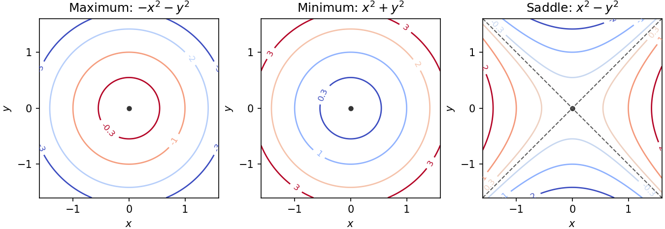
The standard nondegenerate local contour plot models are for a maximum, for a minimum, and for a saddle point of a scalar function. Near a maximum, nested contours have lower values farther from the centre; near a minimum they have higher values. Near a saddle, hyperbolas occur on opposite sides of the critical level, whose contour has two intersecting tangent directions. More general nondegenerate quadratic forms deform these circles into ellipses; degenerate stationary points can have more complicated contours.

Set . The quotient rule gives the partial derivativesSince , the first equation forces . The second then reduces to . Thus the only stationary points and their field values areNo division by a potentially vanishing factor of was used, so no stationary points have been discarded.
The level set can be rearranged, without changing its domain, asThe requested special contours are thereforeThe first is a parabola, the second a single point, and the last two intersecting straight lines. Moreoverwith equality only at . Hence is a strict global maximum. At the crossing critical contour separates sectors with values above and below , so it is a saddle point of a scalar function.
As a Hessian matrix check, is negative definite, while is indefinite. There is no stationary minimum.
For , completing the square gives the conic sectionThe possible levels follow fromFor , the contours are ellipses centred at , shrinking to the maximum as . The zero contour is the parabola from part (c). For , the contours are vertical-opening hyperbolas. At they degenerate into the intersecting straight lines, and for they are horizontal-opening hyperbolas. These descriptions specify the remaining contour families and their symmetry about the axis. The lower bound is approached as at fixed but is never attained.
Contours and an ascending gradient trajectory
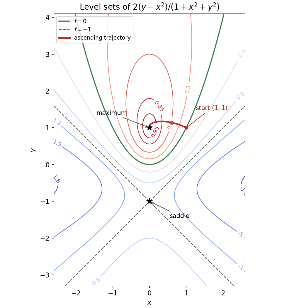
. Original contours of the rational scalar field. The critical points are marked; the green parabola is the zero contour and the crossing dashed lines have level . The red trajectory starts at and follows the positive gradient towards the maximum, as discussed in part (e). Details.
Use the gradient flow of , namely ; any positive change of speed leaves the same trajectory. At the starting point,so the path initially points up and left, with slope . At every regular point it crosses the level sets orthogonally, because the gradient is normal to the contours. Along it,until a stationary point is approached.
The red curve in the plot first rises above , then bends down towards the maximum . It stays on the side and approaches the maximum without crossing it in finite gradient-flow time. Indeed preserves the sign of , and the critical level increases from its starting value towards . The requested curve is an ascending trajectory, not a contour or a straight segment joining the initial and final points.
Split the vector field into and . The second part is the gradient of , so its curl vanishes. The first part has only a vertical curl component, . Hence
The curl found in part (a) is constant, so its divergence isThis also follows from the identity divergence of a curl is zero, applicable here because the field is smooth everywhere.
The original PDF has angle , with an exponent on . It is not : each permitted value of changes the speed but traverses the same circle once counterclockwise. Along the path, andThe radial contribution to the line integral vanishes, since . The rotational contribution givesThereforeThe answer is independent of the monotone parametrization, as an oriented line integral should be.
The upward unit vector extracts the vertical curl component:It is constant over the unit disc, soThis agrees with part (d) by Stokes theorem: the boundary circle has counterclockwise orientation when viewed from the upward normal, including for the parametrizations .
For , differentiate the proposed scalar potential directly:ThusFor , the curl is the nonzero vector . A gradient of a twice differentiable scalar field has zero curl, so no such scalar field exists. Equivalently the closed line integral in part (d) is nonzero, contradicting the path independence of a conservative vector field. The field is smooth on all of , so no excluded singular set complicates this conclusion.
The probability density is symmetric about , vanishes at and , and has its single maximum at . It is zero outside that interval. Its area is one: with the dimensionless change of variablesnormalization is .
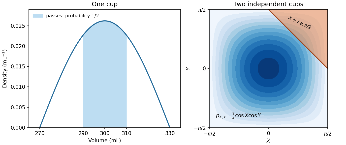

Passing corresponds to in the normalized variable from part (i). Integrating its probability density,The complementary probability of detecting the fault in one test is also .
The absolutely convergent geometric series has sum for . Its Cauchy product with itself isThere are exactly pairs of nonnegative integers whose sum is . Relabeling provesAbsolute convergence justifies the multiplication and regrouping; no differentiation of an infinite series is needed.
Let count tests up to and including the first failure. By independence of random variables, the event requires passes and then a failure. With pass probability and failure probability , this is the geometric distributionUsing part (iii), its expected value isThis counts the test that discovers the fault. The expected number of earlier passing tests alone would be one.
Apply the same dimensionless transformation independently to the two cups, giving . The total-volume condition becomes . Since neither variable can exceed , this region has and , the triangle shown above.
By independence of random variables, the joint probability density is . The desired double integral isThusBoundary equality has probability zero for these continuous random variables.
Because the equation depends on the ratio , set , so . Dividing by and substituting givesThis reduces the homogeneous first-order differential equation to a separable differential equation. For ,At , the condition gives , so and . HenceThe interval displayed is the maximal solution interval containing : there is a pole at . Separating variables omitted the solution , or , but that solution does not satisfy the given condition.
Differentiate once, then substitute the other equation. The required second-order linear differential equation is
The characteristic equation of the homogeneous equation is , giving exponential solutions and . A constant particular solution is . Thus the general solution is
The equation fixes from the same two constants:Indeed , so both original equations hold. No further independent integration constant is available in this two-dimensional linear system of ordinary differential equations.
The dependent variable itself does not occur, so reduce order by putting . Then , a first-order linear differential equation. Its integrating factor is :Integrating once more and renaming the constants givesThe two homogeneous terms are the constant solution and the exponential associated with the roots of the characteristic equation.
For the general solution in part (i),Thus and , giving the solution of the initial value problemDirect substitution checks both the differential equation and the two initial conditions.
The logarithm is defined away from the axis, where . For the vector potential , its curl is . Sincewe obtainFor this is clockwise circulation about the axis, the velocity structure of a point vortex in each transverse plane.
On the same domain, differentiate the Cartesian components:ThusThis is also an instance of divergence of a curl is zero, since the potential is smooth off the axis. The classical field is undefined on the axis, so that identity must not be applied there without specifying an extension.
In cylindrical coordinates, and , soThe potential vector has components . Expanding the prescribed cylindrical curl formula givesThereforeSince , this agrees with the Cartesian result and its clockwise orientation.
The divergence isFor the tetrahedral domain, convenient integration bounds areConsequently its volume integral isPutting , the inner integral is . ThereforeThusThere is an independent centroid check. The vertices are , giving volume and centroid . An affine function averages to its value at the centroid, so . This is the integral of an affine function over a simplex.
Articles were limited to the first 100 out of 140 total.
Articles by others on the same topic
There are currently no matching articles.