Past exam of the mathematics course of the year 1 of the natural sciences course of the University of Cambridge / 2024 / Paper 2 / 14

A displayed minute contains one minute of possible start times, so the specified uniform distribution has probability density functionEndpoint choices for a probability density function do not affect any probabilities.

The graph is a rectangle of height one over $[0,1)$, with zero height elsewhere. Its unit area is the required normalization of the probability density function.

For the uniform distribution, the expected value and second moment areHence the variance is

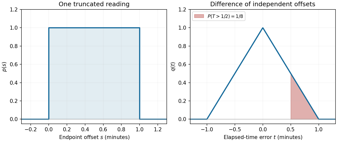
Let $E$ be the finish-time offset from the start of its displayed minute. The elapsed time is $25+E-S$, so $T=E-S$. To obtain the stated density, use the intended model that $E$ and $S$ are independent random variables, both with the uniform distribution on $[0,1)$.

Their joint probability density function is one on the unit square. Equivalently, the convolution of probability densities givesThe integrand is one exactly where $s\in [0,1]$ and $s+t\in [0,1]$. The overlap has length $1+t$ for $-1\le t<0$, length $1-t$ for $0\le t<1$, and zero otherwise. ThereforeThis is a symmetric triangular distribution. The independence and finish-time uniformity are additional modelling assumptions: the two truncated clock readings alone do not imply them. For example, if $E=S$ then the elapsed time is exactly twenty-five minutes and $T=0$, even though each endpoint offset is individually uniform.

The probability density function graph joins $(-1,0)$ to $(0,1)$ to $(1,0)$ and is zero elsewhere, as shown in the right panel of the timing figure. Its area isThus the probability distribution is normalized.

Since $q$ is an even function, $tq(t)$ is an odd function and its integral over the symmetric interval vanishes. Thus $\mathbb{E}[T]=0$. Its variance isConsequentlyThe standard deviation is approximately $0.40825$ minute, or $24.49$ seconds.

An excess of thirty seconds is $T>1/2$ in minute units. ThereforeThis is the shaded triangular area under the probability density function.

The random variable $T$ is the sum $E+(-S)$. The linearity of expectation givesMultiplication by $-1$ reverses the mean but preserves the variance. Under the independence assumption used in part (b), the variance of a sum givesThus both predictions agree with the direct integrals. For the actual elapsed time, adding twenty-five changes the mean to twenty-five minutes and leaves the variance at $1/6$ minute squared.

Without independence, the correct expression is $\mathrm{Var}(T)=1/6-2\mathrm{Cov}(E,S)$ when both marginals are uniform. This explains why independent endpoint errors must be part of the intended model rather than a consequence of the display format.