Equating vector components givesThe third component first forces , then the second forces , and the first gives . ThusEquivalently, the nonzero scalar triple product proves that these three vectors are linearly independent.
The radial coordinate in the cylindrical coordinate system is the Euclidean distance from the -axis:
In spherical coordinates, the radial distance is and . Since the point lies below the equatorial plane, the polar angle exceeds :The angle is approximately radians, or .
For the natural logarithm, . The chord slope is . Hence the mean value theorem point satisfies , givingIt lies strictly between one and two. For example, lies strictly between and one.
The chord through the endpoints is the straight line . At , the tangent line isThese two straight lines have the same slope, as required by the mean value theorem. Since , the natural logarithm is a concave function: its graph lies above the chord and below this tangent line.
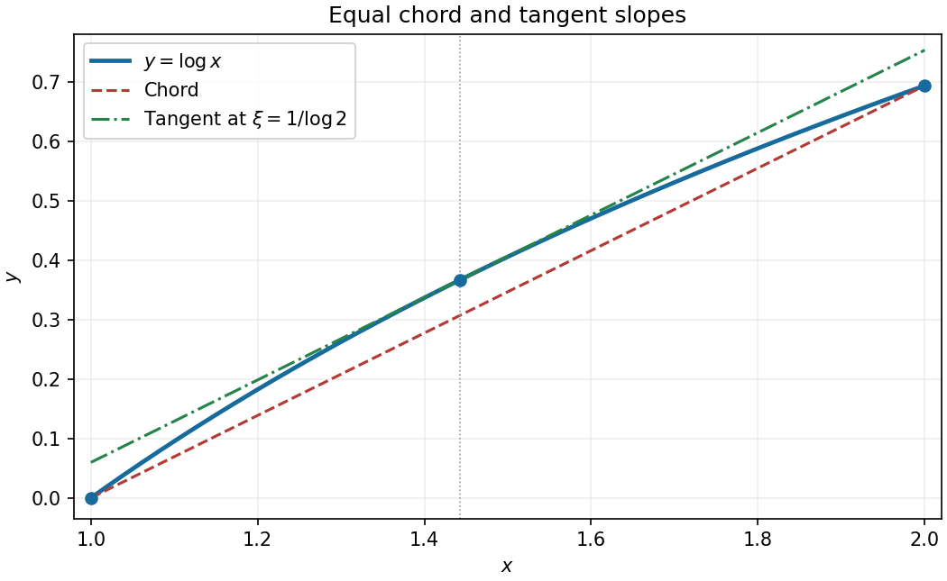
The mean value theorem for the logarithm on the interval from one to two
. The chord and the tangent line at are parallel. The marked point lies on the graph of the natural logarithm. Details.
The fundamental theorem of calculus applies because the integrand is continuous. ThusThe requested derivative is , as shown in the PDF; the local OCR corrupts its notation.
Use the product rule and the fundamental theorem of calculus:Since the integral is , this simplifies to
The Newton root-finding iteration replaces the graph by its tangent line at and uses that line's zero:Comparing with the printed reciprocal-ratio form givesThis step requires . If , the iteration has already reached a zero of a function and the printed reciprocal-ratio expression need not be evaluated.
The addition formula for probability subtracts the overlap, which vanishes for mutually exclusive events:
The chain rule gives , so the given total differential is exact. Thus ; two such functions differ by a constant because their gradient difference vanishes on the connected plane. The assigned value at the origin forces , giving
The divergence of a curl is zero, so its squared absolute value isBoth identities follow by cancellation of equal mixed partial derivatives under the usual smoothness assumptions of vector calculus.
The trigonometric identity gives , and the complementary-angle trigonometric identity gives . Thus the Fourier series is already the finite expressionThe only nonzero Fourier coefficients are and .
The scalar is the signed scalar projection along the unit vector . Multiplying by that unit vector makes the orthogonal projection of onto its span.
For the other expression, the vector triple product identity givesThis is the orthogonal projection onto a plane perpendicular to through the origin. Its dot product with is zero, while the difference from is parallel to .
The two orthogonal projections are complementary, givingThey split a vector into its components parallel and perpendicular to .
The straight line consists of , with . Since the endpoints are distinct, the direction vector can be normalized. ChoosePutting gives the required parametric equation of a straight line . Other choices of on the same straight line, or the opposite direction for , give equivalent descriptions.
Take the cross product with :Thus one choice isConversely, this cross product equation implies , so is parallel to . It therefore describes precisely the original straight line.
The unit vector specifies the direction of the straight line. Reversing its sign, together with the sign of , leaves the same straight line.
Decompose into its orthogonal projections parallel and perpendicular to . Since removes the parallel component,The last vector is the displacement to the point of the straight line nearest the origin. HenceThe original PDF has , not the squared magnitude inserted by the OCR.
The vector is a normal vector to the span of and . Since , these vectors determine a plane. Thus the missing words are
the line and the origin.
A necessary compatibility condition is , because a cross product with is perpendicular to it. If this condition fails, there is no solution.
If it holds, take the equation and use the vector triple product identity:Thus the perpendicular orthogonal projection is fixed and the parallel component is free:Conversely, under the compatibility condition, so every displayed vector solves the equation. The solution set is a straight line, including the line through the origin when .
The gradient is horizontal when and vertical when . Factoring those partial derivatives gives the two loci:Thus each locus consists of an axis and two parabolas. Their common points are the five stationary points found below. At those points the gradient is zero and has no direction, so they are included in both algebraic zero-component conditions but excluded if “parallel” is required to mean a nonzero directed vector.
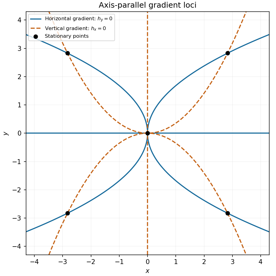
Loci of horizontal and vertical gradients
. Blue curves have , orange curves have , and black points mark their intersections. At the black points the gradient itself vanishes. Details.
A stationary point must satisfy both factored equations from part (a). If either coordinate is zero, the other equation forces the other coordinate to vanish. This gives .
Otherwise and . With and , these become and . Dividing gives , so . Then forces . Hence all five stationary points are
The Hessian matrix isAt each nonzero stationary point, its diagonal entries are and the off-diagonal entries are . Its eigenvalues are and , both positive. Thus the Hessian matrix is positive definite, and the second-derivative test proves thatTheir common value is . In fact they are global minima: with , the arithmetic-geometric mean inequality gives , soThe last one-variable polynomial attains its minimum at , and equality in the first bound requires , precisely the four points above.
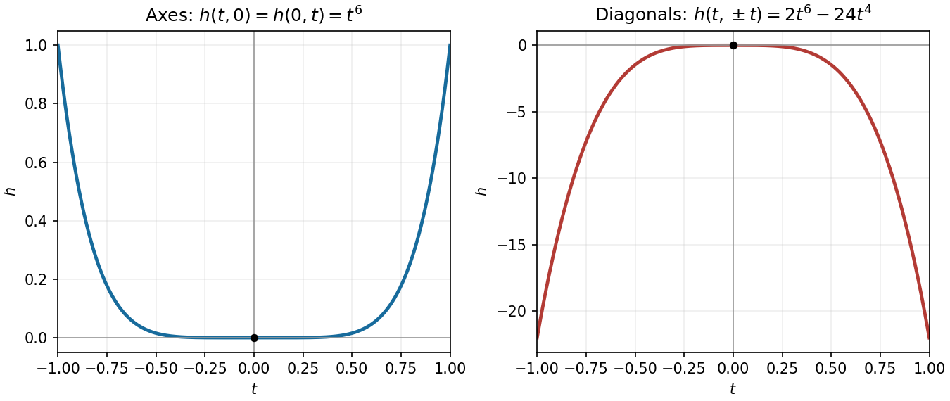
Along either coordinate axis, the restriction is , which is positive for . Along either diagonal it iswhich is negative for sufficiently small nonzero . Therefore every neighbourhood of the origin contains both positive and negative values, whereas . ConsequentlyThe Hessian matrix vanishes there, so the ordinary second-derivative test is inconclusive; the restrictions settle the question.

Near a nonzero stationary point , Taylor expansion of the gradient gives . Since the Hessian matrix is positive definite, for sufficiently small nonzero . Thus the gradient arrows point away from each of the four local minima, with different strengths in the two eigenvector directions.
At the origin, on the -axis the gradient is and on the -axis it is , so arrows point outward. On the gradient is , and on it is , so arrows point toward the origin for small . Away from the axes the leading terms are , pointing inward in both coordinate signs. The narrow outward sectors close to the axes are visible in the exact vector field.
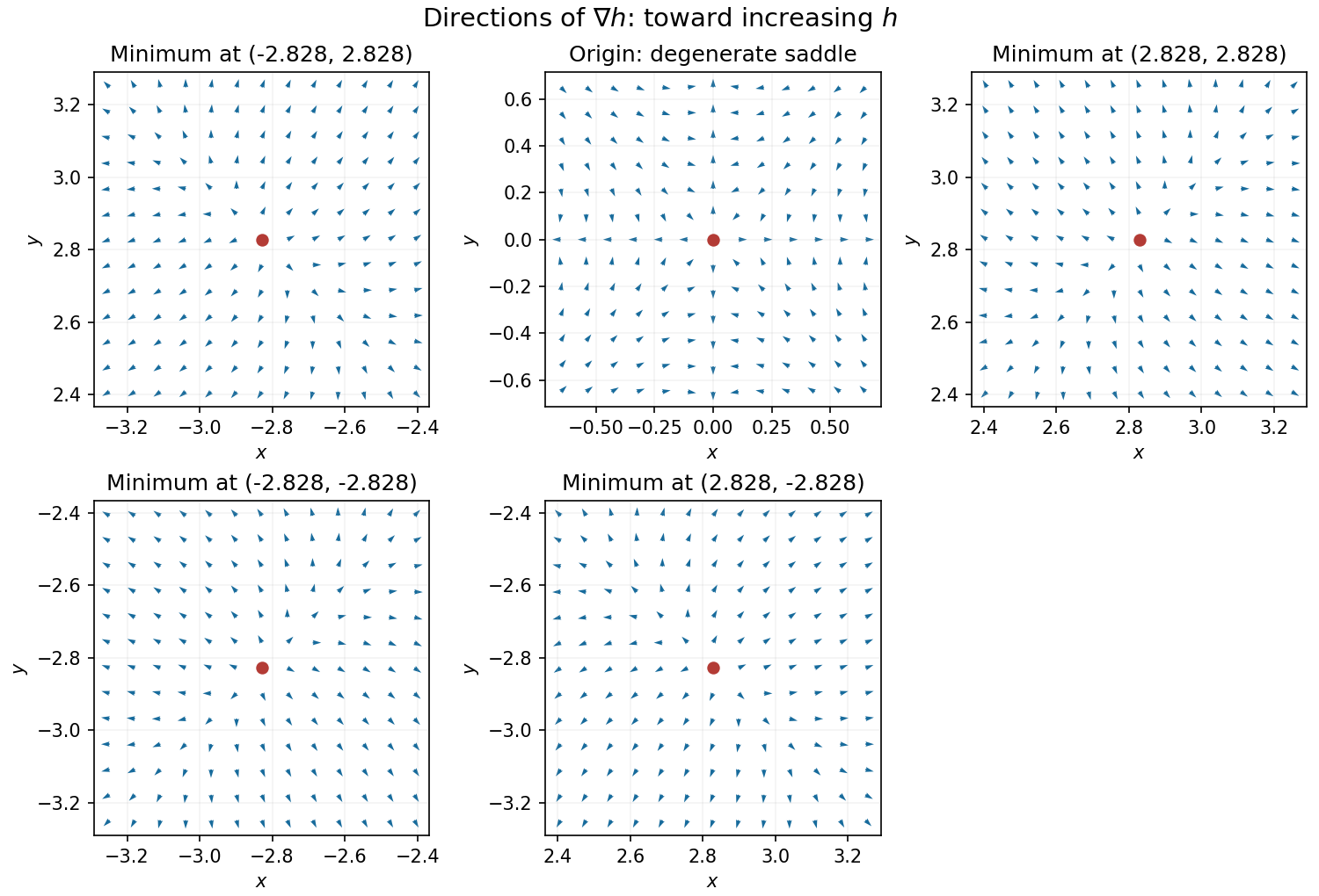
Gradient directions near all five stationary points
. Arrows show normalized gradient directions, not the direction of descent. They point outward near the four minima, while the degenerate origin has outward axis directions and inward diagonal directions. Details.
For , the product rule for the curl givesSince , this is not identically zero on . A gradient field has zero curl, so no scalar potential exists for on the whole space.
For the radial vector field , observe thatThus all vector-field potentials areThese are smooth everywhere, including the origin. Any two differ by a constant because their gradient difference vanishes on the connected whole space.
On the circular arc, and , so the line integral reduces toThis exact differential evaluation applies to the specified arc; for example its parametric equation is , . On the vertical segment , only contributes, giving . The whole path therefore givesTo answer the final conservativeness requirement, compute the curl:It vanishes identically exactly whenOn the simply connected whole space this condition is sufficient for a conservative vector field. Explicitly a vector-field potential isBoth path calculations then give , equal to by the fundamental theorem for line integrals. Equality of just these two path values would only force ; it is the curl calculation that establishes full path independence.
A displayed minute contains one minute of possible start times, so the specified uniform distribution has probability density functionEndpoint choices for a probability density function do not affect any probabilities.
The graph is a rectangle of height one over , with zero height elsewhere. Its unit area is the required normalization of the probability density function.
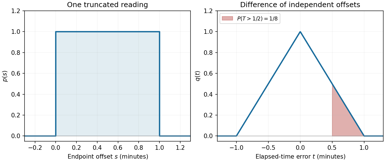

Let be the finish-time offset from the start of its displayed minute. The elapsed time is , so . To obtain the stated density, use the intended model that and are independent random variables, both with the uniform distribution on .
Their joint probability density function is one on the unit square. Equivalently, the convolution of probability densities givesThe integrand is one exactly where and . The overlap has length for , length for , and zero otherwise. ThereforeThis is a symmetric triangular distribution. The independence and finish-time uniformity are additional modelling assumptions: the two truncated clock readings alone do not imply them. For example, if then the elapsed time is exactly twenty-five minutes and , even though each endpoint offset is individually uniform.
The probability density function graph joins to to and is zero elsewhere, as shown in the right panel of the timing figure. Its area isThus the probability distribution is normalized.
Since is an even function, is an odd function and its integral over the symmetric interval vanishes. Thus . Its variance isConsequentlyThe standard deviation is approximately minute, or seconds.
An excess of thirty seconds is in minute units. ThereforeThis is the shaded triangular area under the probability density function.
The random variable is the sum . The linearity of expectation givesMultiplication by reverses the mean but preserves the variance. Under the independence assumption used in part (b), the variance of a sum givesThus both predictions agree with the direct integrals. For the actual elapsed time, adding twenty-five changes the mean to twenty-five minutes and leaves the variance at minute squared.
Without independence, the correct expression is when both marginals are uniform. This explains why independent endpoint errors must be part of the intended model rather than a consequence of the display format.
The characteristic equation has the repeated polynomial root , because both and occur as independent solutions. Hence its characteristic polynomial isComparing constant terms gives
Articles were limited to the first 100 out of 163 total.
Articles by others on the same topic
There are currently no matching articles.