Differentiate the spatial Fourier transform under the integral, and integrate the second spatial derivative by parts twice. For sufficiently decaying temperature and first derivative, the boundary terms vanish:Hence the transformed heat equation is the ordinary differential equation
Solving the transformed ordinary differential equation with its initial condition gives . The Fourier inversion theorem therefore yieldsFor the Gaussian multiplier suppresses large spatial frequencies, which explains the smoothing produced by heat conduction.
The convolution theorem turns the product into a spatial convolution. Its kernel isComplete the square:After rescaling the variable, the supplied translated Gaussian integral givesThis is the heat-kernel solution for diffusivity one. Its kernel integrates to one, preserving the total temperature integral, and approaches a Dirac delta function as . Its variance is ; the factor is appropriate to , rather than the alternative convention with diffusivity .
For the Gaussian initial data for the heat equation, substitute the initial profile into the heat-kernel solution. Completing the square in givesThe remaining Gaussian integral yieldsThe centre stays at and the squared width grows linearly with time.
For the interval pulse, the convolution reduces to . Using and the error function givesThis is the translated and scaled heat equation with interval-indicator initial data. At its jump points the limits are ; away from them the initial data are recovered pointwise.
For fixed at late time, both error function arguments are small. Since ,The estimate is uniform for . Equivalently, on this fixed interval the Gaussian in the convolution is .
The spreading distance is more apparent on the growing spatial scale. For the Gaussian pulse the exponent is order one when . For the interval pulse, set with and fixed . Uniformly for bounded , its convolution givesThus both nonzero pulses spread over a distance , while their heights are and their total integrals remain constant. More quantitatively, the variances of their normalized profiles are and , respectively, confirming the same width law.
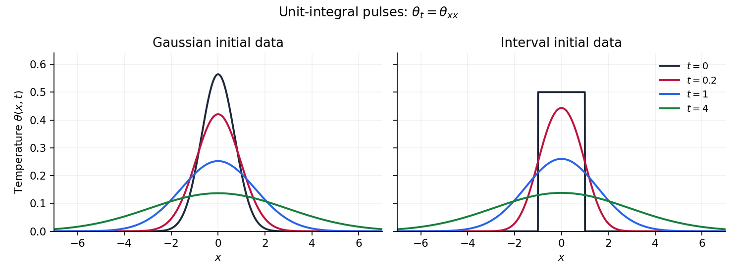
Gaussian and interval initial profiles broaden under the heat equation while conserving their integrals
. Details. 
Articles by others on the same topic
There are currently no matching articles.