Thermal conduction transfers heat through microscopic interactions without bulk transport of matter. To predict the heating load through a bar, combine Fourier's law with conservation of energy and the imposed end temperatures. In the isotropic model with positive thermal conductivity , the conductive heat flux points from high to low temperature, opposite to the temperature gradient. A spoon warming along its handle and heat escaping through a wall are familiar examples.
Consider a bar of length , constant cross-sectional area and constant thermal conductivity . Maintain its ends at and , with increasing toward the colder end. Assume a steady state, one-dimensional thermal conduction, no internal sources and no heat transfer through the sides. The temperature falls by over , givingThe difference between the two readings in degree Celsius units is the same -kelvin difference. The positive heat flux carries heat toward increasing .
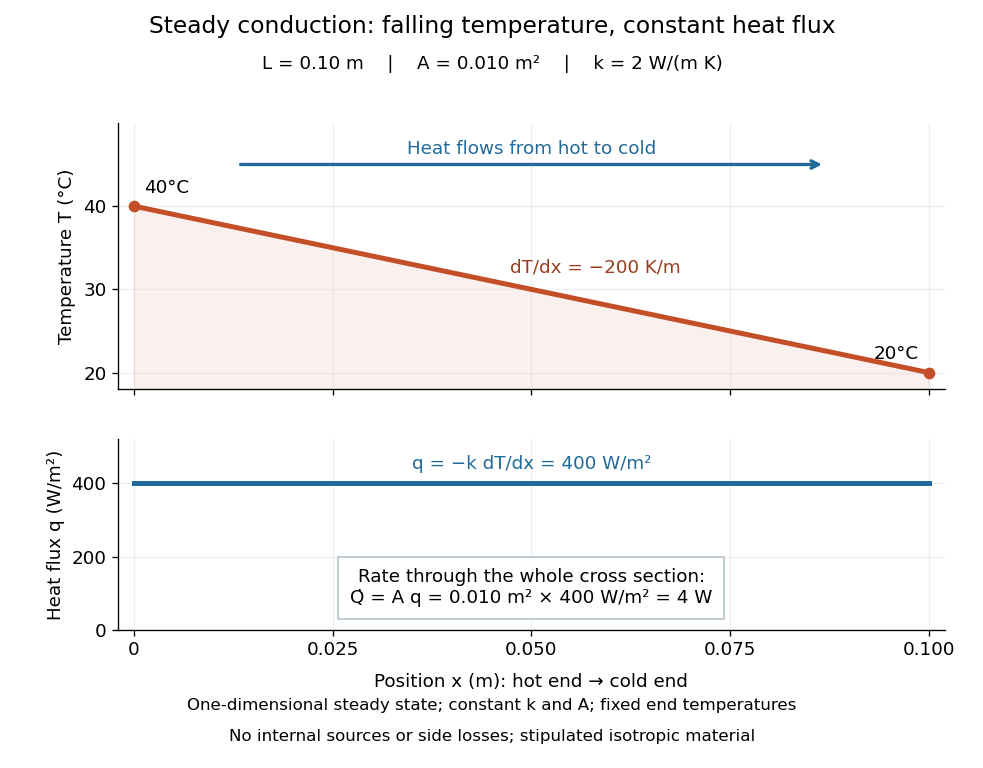
The general solution under these assumptions isA proof outline is enough to explain the straight line: conservation of energy in any small slice, with no accumulation, sources or side losses, gives . Constant cross-sectional area gives ; constant thermal conductivity and Fourier's law then give . Two integrations and the end boundary conditions determine the displayed affine function. This is why a visually simple temperature profile can encode a continuous flow of energy. [ref]
https://web.mit.edu/16.unified/www/FALL/thermodynamics/notes/node117.html. E. M. Greitzer, Z. S. Spakovszky and I. A. Waitz, MIT Thermodynamics and Propulsion, section 16.3: steady one-dimensional conduction
Doubling the length halves the rate, while doubling the cross-sectional area doubles it, at fixed end temperatures and thermal conductivity. This explains why a long narrow support can limit unwanted heat transfer, while a short broad path can help remove heat. Joining materials leads to thermal resistance in series. During initial warming, internal energy can accumulate and the temperature profile need not be a straight line; the time dependence is described by the heat equation and thermal diffusivity.
Now join two layers, each of length , with constant cross-sectional area and stipulated constant thermal conductivities and . Keep the outer ends at and . Assume a steady state, one-dimensional thermal conduction, no internal sources or side losses, and perfect contact: the temperature is continuous at the interface, with no extra contact drop. For each layer, use the area-specific thermal resistance and . The series calculation gives
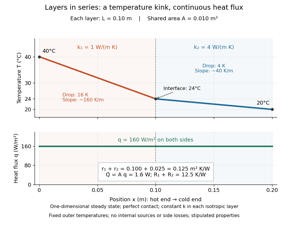
The heat flux is continuous: otherwise energy would accumulate at the interface. Yet Fourier's law gives different temperature gradients, and . Lower thermal conductivity requires a steeper temperature gradient to carry the same heat flux; equal lengths therefore give drops in the ratio . A kink in the temperature profile records the change of material while perfect contact keeps the temperature itself continuous.
Thermal resistance measures the temperature drop required to drive a given rate of heat transfer. For the steady one-dimensional bar model in thermal conduction,Here relates the temperature drop to heat flux, while relates it to the rate of heat transfer. The single bar above has and , so its drop drives .
To see why series thermal resistances add, apply Fourier's law in each layer to obtain . With no accumulation or side losses the rate of heat transfer is the same through both, so adding the drops gives . This lets us size layered walls without solving a new differential equation for every layer. The structure matches Ohm's law: temperature difference plays the role of electric potential difference, the rate of heat transfer plays the role of electric current, and thermal resistance plays the role of electrical resistance. [ref]
https://web.mit.edu/16.unified/www/FALL/thermodynamics/notes/node118.html. E. M. Greitzer, Z. S. Spakovszky and I. A. Waitz, MIT Thermodynamics and Propulsion, section 16.4: series thermal resistances and the electrical analogy
In the absence of heat advection, an insulating sphere of radius in a uniform remote temperature gradient has the displayed exterior harmonic function as its temperature field. The reflected dipole term makes at . The surface temperature is , so the tangential gradient is amplified by . If the sphere has thermal conductivity ratio relative to its surroundings, temperature and heat-flux continuity instead give surface gradient factor .
With fixed pressure , let , so . A material mass coordinate has and the material time derivative becomes . The energy and continuity equations then give the displayed equation with and . A mass integral from a fixed origin is material only when the mass flux there vanishes; otherwise subtract its time-integrated flux to label parcels. Uniform pressure is a low-Mach approximation when sound crossing is faster than thermal evolution.
For conductivity , no cooling in the hot phase and a zero-temperature boundary at , the mass-coordinate equation is linear diffusion. Its similarity profile solves , , , giving the displayed error function. The thermal layer broadens as the square root of time. Conducted energy enters the cold radiating reservoir at rate per area , hence .
The temperature gradient is the gradient of the temperature field. It points in the direction of fastest temperature increase.
Fourier's law predicts the local conductive heat flux from the local temperature gradient. In a continuum approximation with isotropic thermal conductivity , its vector form and one-dimensional form areThe heat flux has units , the temperature gradient has units and the thermal conductivity has units . The rate of heat transfer has units . These units distinguish a local material response from the total power crossing a surface.
The minus sign makes heat flow toward lower temperature: for , . In the worked bar in thermal conduction, therefore gives . Reversing the end temperatures reverses the heat flux. A zero temperature gradient gives zero conductive heat flux in this model.
Fourier's law is a constitutive relation expressing measured material behavior; it is not a consequence of conservation of energy alone. It applies locally and does not require a steady state. The straight-line bar solution additionally assumes constant thermal conductivity, constant cross-sectional area, no sources or side losses, and fixed end temperatures. Anisotropic materials require the directional response described by the thermal conductivity tensor. The scalar used in the examples expresses the stated isotropy assumption. [ref]
https://web.mit.edu/16.unified/www/FALL/thermodynamics/notes/node116.html. E. M. Greitzer, Z. S. Spakovszky and I. A. Waitz, MIT Thermodynamics and Propulsion, section 16.2: Fourier's law and thermal conductivity
Historically, Joseph Fourier's Théorie analytique de la chaleur was published in 1822. In Chapter II, article 112, he writes the heat crossing a spherical surface as the product of thermal conductivity, elapsed time, surface area and the negative radial temperature gradient; article 113 balances the incoming and outgoing heat to obtain the heat equation for a sphere. The enduring idea is this connection between a local flow rule and a global prediction of changing temperature. [ref]
https://fr.wikisource.org/wiki/Théorie_analytique_de_la_chaleur. Joseph Fourier, Théorie analytique de la chaleur, Firmin Didot, 1822
[ref]https://fr.wikisource.org/wiki/Théorie_analytique_de_la_chaleur/Chapitre_2. Fourier, 1822, Chapter II, articles 112–113
Thermal conductivity is the material response coefficient in Fourier's law. For an isotropic material it is a scalar , with units ; larger positive means a larger conductive heat flux for the same temperature gradient. It can depend on temperature and composition. Direction-dependent response in an anisotropic material is described by a thermal conductivity tensor. The two worked examples use stipulated positive constants, rather than measured values for named materials.
Thermal conductivity describes material response, whereas thermal resistance also includes geometry: for the steady bar, . Doubling at fixed length, cross-sectional area and end temperatures halves thermal resistance and doubles the rate of heat transfer. Doubling length changes thermal resistance without changing the material's thermal conductivity. This distinction lets a designer improve cooling either by choosing a higher thermal conductivity or by shortening and widening the path. It also explains why the less conductive layer in thermal resistance takes the greater temperature drop.
Thermal diffusivity answers a different question: how rapidly a temperature disturbance spreads. Its usual model also involves mass density and specific heat capacity , so equal thermal conductivities need not imply equal rates of warming.
The thermal conductivity tensor maps a temperature gradient to the negative heat-flux density. In passive reciprocal conduction it is symmetric positive definite. This permits direction-dependent transport while ensuring positive dissipated energy.
Thermal diffusivity measures how rapidly thermal conduction smooths a temperature difference inside a material. Thermal conductivity measures the heat flux driven by a specified temperature gradient; thermal diffusivity also accounts for the heat capacity that must be warmed. A material can carry substantial heat yet change temperature slowly because it stores substantial internal energy per kelvin.
Write for thermal diffusivity, reserving for thermal conductivity. In a homogeneous isotropic material,Here is mass density, is specific heat capacity for the relevant mechanical constraint, and is volumetric heat capacity. The familiar uses specific heat capacity at constant pressure. For ordinary solids with negligible thermal expansion, the difference between the two constrained specific heat capacities is often neglected. A rigid fixed-volume model instead uses specific heat capacity at constant volume; a compressible moving fluid requires the accompanying work and transport terms. Thus the constraint is part of the approximation, not a choice made solely from the units. [ref]
Light and Laser Flash Analyzers by NETZSCH Analyzing and Testing. NETZSCH, Principle of the LFA Method: conductivity equals diffusivity times specific heat capacity times density
Assume a stationary material in the continuum approximation, local thermal equilibration on times shorter than those resolved, no internal heating, no phase transition, and negligible convection and mechanical work. Combining conservation of energy with Fourier's law gives the one-dimensional balanceIf are constant over the region and temperature excursion, this becomes the heat equation . If varies, retain the differentiated product; replacing it with loses a term. Anisotropic materials need a thermal conductivity tensor. The scalar constant- examples below deliberately exclude these complications. [ref]
Rear-surface integral method for calculating thermal diffusivity from laser flash experiments by Elliot J. Carr. Carr, section 1: homogeneous isotropic constant-property assumptions; section 2, equations (1)–(3): insulated one-dimensional heat equation
For an original comparison, stipulate two model materials with equal thermal conductivity and equal mass density , but specific heat capacities and . ThenAt the same temperature gradient, both have the same instantaneous heat flux by Fourier's law. At the same initial temperature profile and boundary conditions, material B takes four times as long to smooth a given spatial pattern. With fixed end temperatures, identical geometry and no sources, both eventually have the same steady profile and heat flux. The larger heat capacity changes the transient, not this steady state. These are stipulated parameters, not measurements of named substances.
The Prandtl number is the ratio of kinematic viscosity to thermal diffusivity. It compares the rates at which momentum and temperature variations diffuse. In thermal-diffusion units the Boussinesq equations have momentum inertia multiplied by ; large, rather than small, Prandtl number supplies the usual instantaneous Stokes flow limit.
The thermal diffusion time , with the thermal diffusivity, is a characteristic scale for smoothing a temperature variation over length . It is the thermal instance of the diffusive time scale. Rescaling and removes and from the constant-coefficient heat equation. Doubling length therefore multiplies comparable internal equilibration times by four; increasing thermal diffusivity by four divides them by four.
This scale is not a universal time of complete thermal equilibrium. A nonzero Fourier mode decays exponentially and never becomes exactly zero at finite time. The geometry, boundary conditions, initial pattern and accepted residual determine the numerical factor. For example, an insulated bar's slowest nonuniform Fourier mode has decay time , and reducing its amplitude to a fraction requiresExternal heat transfer can impose a longer cooling time even when internal temperature differences smooth quickly. Thermal diffusivity alone does not determine cooling to the room's temperature.
With thermal diffusivity , a Fourier mode of angular wavenumber decays at rate . To avoid confusing this with thermal conductivity, use and angular wavenumber below: the same rate is , with units .
Consider an insulated bar with constant thermal diffusivity, no sources and no heat flux through either end or the sides. An original initial temperature profile and its exact evolution areThe cosine has zero temperature gradient at both ends, satisfying the insulated Neumann boundary conditions. Its spatial mean is zero, so conservation of energy leaves the mean temperature unchanged while the nonuniform part disappears. A short derivation substitutes into the heat equation: the second spatial derivative supplies , hence . The exponential decay time is ; doubling angular wavenumber quarters this time. If cycles-per-length spatial frequency is used instead, and the rate is .
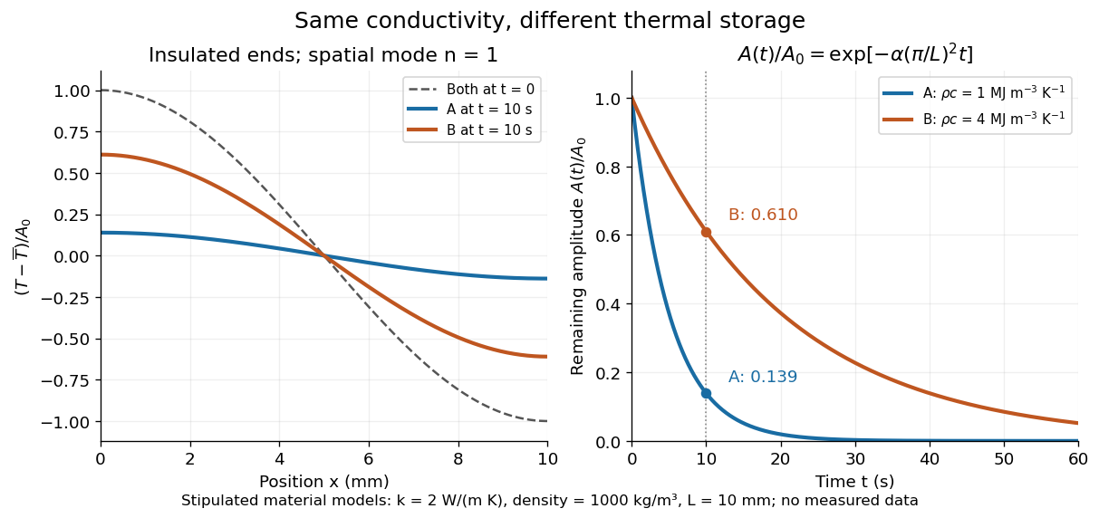
For the two model materials in thermal diffusivity and , and . After , the remaining amplitude fractions are approximately and . A narrow hot-and-cold pattern disappears faster than a broad one because its temperature curvature, and hence the imbalance in conductive heat flux, is larger.
The thermal diffusion length is the characteristic length over which thermal conduction changes a temperature distribution during time in the constant-thermal diffusivity model. It is a scale, not a sharp front or distance travelled at a constant speed: the heat equation has infinite propagation speed mathematically. Different definitions of penetration depth introduce numerical factors. In particular, the normalized one-dimensional heat kernel has spatial variance , so its root-mean-square width is .
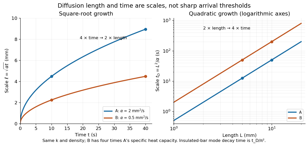
Thermal diffusion length grows as the square root of time; thermal diffusion time grows as length squared
. Original predictions for the two stipulated materials in thermal diffusivity. Left: , with four times the time needed to double length. Right: on logarithmic axes. Equal thermal conductivity with four times the volumetric heat capacity halves the reached length at a given time and quadruples the time at a given length. The scale differs from the insulated-bar decay time by the factor . Details.At , the model materials have thermal diffusion lengths and . For their thermal diffusion times are and . These values describe the same heat equation as the thermal diffusion rate of a Fourier mode; the different numerical factors come from the definition of the scale.
Laser flash analysis measures thermal diffusivity by heating one face of a specimen briefly and recording the opposite face's temperature rise. The original 1961 experiment used a flash tube rather than a laser: a blackened thin metal specimen sat in an opaque ceramic holder, with thermocouple wires pressed against its rear face. An amplifier, oscilloscope and camera recorded the signal. Uniform front illumination and the black coating promoted uniform absorption; the opaque low-thermal conductivity holder blocked direct rear illumination and reduced edge losses. The delayed rear response reveals internal thermal conduction rather than direct heating of the sensor. [ref]
Flash Method of Determining Thermal Diffusivity, Heat Capacity, and Thermal Conductivity by W. J. Parker and others. Parker, Jenkins, Butler and Abbott, pp. 1682–1683, Experimental Procedure and figure 3: holder, flash, thermocouple and recording chain
A modern version uses a laser or flash lamp, a specimen of measured thickness , controlled initial temperature, and a rear-facing infrared detector with a synchronized recorder. The readout is a temperature rise versus time, starting from a pre-pulse baseline. Thermal conductivity additionally requires mass density and specific heat capacity; it is not obtained from timing alone. [ref]
Light and Laser Flash Analyzers by NETZSCH Analyzing and Testing. NETZSCH, Principle of the LFA Method: opposite-face infrared readout and conductivity product
Under ideal one-dimensional, insulated, constant-property assumptions, instantaneous uniform absorption in a very thin front layer gives the normalized rear riseHere is the initial uniform temperature and is the final uniform temperature in the insulated model. Fitting this curve estimates thermal diffusivity; each term has the same decay as the insulated-bar Fourier modes. Equivalently, the half-rise time solves . Writing , the series gives , henceThis coefficient comes from the stated ideal heat equation solution, not from an empirical sensor calibration. It has been independently checked by solving the series equation. Absolute absorbed pulse energy cancels from the normalized curve; determining heat capacity from its absolute height needs additional information. [ref]
Parker and colleagues identify finite flash duration, heat loss, nonuniform illumination, recording bandwidth and electrical interference as practical limits. A specimen too thin responds during the pulse; one too thick allows losses before the rear rise finishes. They shielded the electrical chain and recorded a baseline; their reported tests were preliminary metal measurements near ambient and moderately elevated temperatures. [ref]
Flash Method of Determining Thermal Diffusivity, Heat Capacity, and Thermal Conductivity by W. J. Parker and others. Parker and colleagues, pp. 1682–1684: signal distortion, shielding, thickness tradeoff and Conclusions
Useful additional controls are to measure thickness at several points, verify the recorder's time scale and detector response independently, record a no-pulse baseline, and repeat at different pulse energies while avoiding phase transitions. Compare different thicknesses of the same homogeneous material: ideal half-rise times scale as . Failure of these checks can expose finite-pulse effects, sensor delay, optical transmission, coating storage or edge losses; a thickness error is especially consequential because the inferred thermal diffusivity depends on . These are proposed diagnostic controls, not invented measurements. When the pulse is not short or the sample exchanges appreciable heat with its surroundings, fit a model that includes those effects instead of applying the ideal half-rise coefficient unchanged.
Articles by others on the same topic



Thermal conduction is the process by which heat energy is transferred through materials without any flow of the material itself. This transfer occurs due to temperature differences within a substance or between different substances in thermal contact. When a region of a material is heated, the particles in that region gain energy and vibrate more vigorously. These excited particles collide with neighboring particles, transferring some of their energy to them, which raises their temperature. This process continues, allowing heat to move from the hotter area to the cooler area.