Multiplying by makes the first two terms a total derivative:The resulting Sturm-Liouville form isEquivalently, an integrating multiplier must satisfy , which reduces to and gives up to a constant. The coefficient is positive for and vanishes linearly at the left endpoint; the weight is positive throughout. The boundedness condition removes the logarithmic local branch, giving the no-log boundary condition at a linearly vanishing Sturm-Liouville endpoint.
The appropriate weighted inner product and Sturm-Liouville operator areFor two functions obeying the endpoint conditions, integration by parts gives the Lagrange identity for a Sturm-Liouville operatorAt , both and vanish. At , the factor tends to zero while the functions and their first derivatives remain bounded. Thus the boundary form vanishes at both ends.
This gives the regular self-adjoint differential operator realization: its singular-end condition is , together with . The bounded classical eigenfunctions satisfy exactly this no-log choice. More precisely the operator domain is the maximal differential-operator domain in the weighted space with these separated endpoint conditions; the preceding calculation verifies its self-adjoint boundary form, rather than merely the differential expression's formal symmetry.
Let be an eigenfunction, allowing complex values for the reality argument. The self-adjoint differential operator identity and integration by parts giveThe boundary term vanishes for the same reasons as in part ii. The denominator is real and positive; the numerator is real and strictly positive because and . Hence the Rayleigh quotient isThe positivity uses a nondegenerate interval .
For real eigenfunctions , multiply their Sturm-Liouville problems crosswise and subtract. Integration givesAt , both eigenfunctions vanish, while at their bounded values and bounded first derivatives multiply a factor tending to zero. The right side is zero. Distinct eigenvalues therefore give the orthogonality of Sturm-Liouville eigenfunctionsFor complex eigenfunctions, replace by , in accordance with the weighted inner product.
Use separation of variables, , in the Laplace equation in polar coordinates. Dividing by givesSingle-valued -periodic angular factors have integer . For , they are , and the radial equation has solutions . The zero angular mode gives . These separated products give the requested solutions; arbitrary sums may use independent coefficients for each radial-angular combination.
Boundedness at the origin removes the logarithm and all negative radial powers. The boundary function is even, so its sine Fourier coefficients vanish. With the convention , its Fourier coefficients areThus the bounded interior harmonic extension isFor the series and its derivatives converge locally uniformly, so it is harmonic. It is a rotated and scaled instance of the harmonic measure of a semicircle in a disk. For example, summing the power series for the complex arctangent, or differentiating the following expression, gives the equivalent real formThis also proves boundedness directly.
At the two jumps, the boundary interpretation matters. At every continuity point the radial limit equals the prescribed value. At , the radial limit is , the midpoint of the two one-sided values. Consequently for there is no harmonic solution continuous on the closed disk with exactly the printed boundary values. The standard bounded Dirichlet problem imposes the trace away from the jumps, or almost everywhere; assigning zero separately at those two boundary points does not alter the interior solution.
For uniqueness let . Formally the divergence theorem applied to givesFor continuous zero boundary data, this immediately forces . With the actual discontinuous data, one should justify the two exceptional points rather than assume finite Dirichlet energy there. Let and choose a cutoff which is zero within of those points, one beyond , and linear in logarithmic distance between. Its gradient satisfies . Applying the divergence theorem to givesThe resulting energy tends to zero. Hence on every compact subset and is constant; its zero boundary trace on the open arcs makes it zero. This is the logarithmic cutoff proof of harmonic uniqueness with finitely many boundary exceptions.
For the exterior harmonic extension of disk boundary data, boundedness instead excludes and the logarithm. The same boundary coefficients giveThis is , using inversion in a circle. Its limit at infinity is . To see why that value is forced independently of this construction, average any bounded exterior harmonic function over a circle. The mean satisfies , hence is . Boundedness forces , and the boundary mean fixes . A constant limit at infinity must therefore be .
Finally suppose two bounded exterior solutions have this limit. Their difference tends to zero. Under planar inversion in a circle, it is bounded and harmonic near the origin, so the isolated point there is removable. Its local expansion gives , in the original exterior. Apply the preceding divergence theorem energy argument on , with logarithmic cutoffs at the two boundary jumps. After removing those cutoffs, the inner boundary term vanishes; the outer one is . Letting forces , and the zero limit gives . Thus the bounded exterior solution is unique as well.
The outgoing Green function for the three-dimensional Helmholtz equation satisfiesIts normalization follows by integrating over a small ball about : , so its outward derivative has flux . Apply Green's second identity in the variables:The terms cancel. Thus the surface integral equals for , and zero for outside the closed volume. Equivalently, remove a small source ball and evaluate its flux before taking its radius to zero. A source on the boundary would require a different limiting formula and is not part of this calculation.
For the upper half-space, take a half-ball of radius . Interpret the first far-field condition as , and the radiation limit in its usual direction-uniform sense, namely the Sommerfeld radiation conditionThis is the finite-bound interpretation of the PDF's first condition. For fixed and real ,Indeed , and its radial derivative is . On the large hemisphere the integrand can therefore be rewritten asIts area is , so its integral tends to zero. The planar integral, taken over expanding disks if needed, consequently equals for and zero for .
The outward unit normal vector on the bottom plane is . Denote this planar integral byFor reflect the source point to . On the plane,Adding and cancels the boundary values of and gives . Thus the Neumann representation for a radiating Helmholtz half-space isThe negative sign is consistent with using the upward derivative rather than the outward normal derivative. If that upward derivative is zero everywhere on the plane, the integral is zero. Hence throughout the upper half-space in the specified radiating class; taking a difference also gives uniqueness for prescribed Neumann boundary data.
Put and . The denominator of the complex rational function becomesThe quadratic formula gives its two zeros, hence the two poles:Their product is , so . To locate them one also needs to exclude the possibility of both lying on the unit circle. Here their moduli are explicit:Both are simple poles: takes the nonzero values and at them. In particular their residues are and .
For the real integral, use the change of variables . As runs from to , this traverses the unit circle once counterclockwise, andThus . Only is enclosed. The residue theorem, or Cauchy integral formula after subtracting its simple-pole part, givesThe real denominator is positive because . As an independent check, write ; a period shift reduces the answer to the existing reciprocal affine sine integral.
Differentiate the spatial Fourier transform under the integral, and integrate the second spatial derivative by parts twice. For sufficiently decaying temperature and first derivative, the boundary terms vanish:Hence the transformed heat equation is the ordinary differential equation
Solving the transformed ordinary differential equation with its initial condition gives . The Fourier inversion theorem therefore yieldsFor the Gaussian multiplier suppresses large spatial frequencies, which explains the smoothing produced by heat conduction.
The convolution theorem turns the product into a spatial convolution. Its kernel isComplete the square:After rescaling the variable, the supplied translated Gaussian integral givesThis is the heat-kernel solution for diffusivity one. Its kernel integrates to one, preserving the total temperature integral, and approaches a Dirac delta function as . Its variance is ; the factor is appropriate to , rather than the alternative convention with diffusivity .
For the Gaussian initial data for the heat equation, substitute the initial profile into the heat-kernel solution. Completing the square in givesThe remaining Gaussian integral yieldsThe centre stays at and the squared width grows linearly with time.
For the interval pulse, the convolution reduces to . Using and the error function givesThis is the translated and scaled heat equation with interval-indicator initial data. At its jump points the limits are ; away from them the initial data are recovered pointwise.
For fixed at late time, both error function arguments are small. Since ,The estimate is uniform for . Equivalently, on this fixed interval the Gaussian in the convolution is .
The spreading distance is more apparent on the growing spatial scale. For the Gaussian pulse the exponent is order one when . For the interval pulse, set with and fixed . Uniformly for bounded , its convolution givesThus both nonzero pulses spread over a distance , while their heights are and their total integrals remain constant. More quantitatively, the variances of their normalized profiles are and , respectively, confirming the same width law.
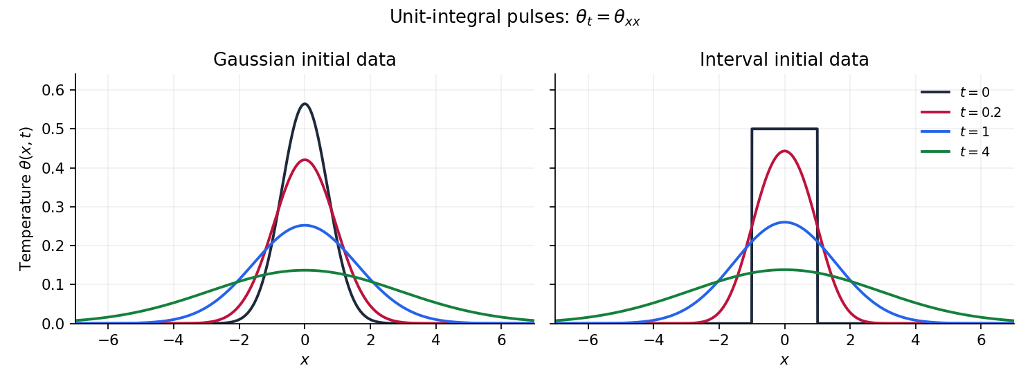
Gaussian and interval initial profiles broaden under the heat equation while conserving their integrals
. Details. 
In Cartesian coordinates a rank- tensor is an array whose components transform under a change of orthonormal axes by one rotation matrix factor per index:An isotropic tensor has unchanged components under every proper rotation. The Levi-Civita symbol obeysfor , proving rotation invariance of the Levi-Civita symbol. Under an orthogonal transformation of determinant its sign reverses; including such transformations requires the pseudotensor distinction. Here isotropy is with respect to proper rotations.
Contract the determinant identity with . Since , one obtainsEvery index on the right is contracted, so the tensor component transformation law leaves no free rotation factor: the determinant is a scalar. Equivalently, gives .
For the matrix inverse, defineThis is the cofactor matrix. To verify the inverse formula rather than just recognize it, contract with and use the determinant identity again:Here the contraction of two Levi-Civita symbols gives . Therefore and, when ,These are the Levi-Civita formulas for a three-dimensional determinant and inverse.
Now differentiate the cubic determinant formula with respect to the individual entry . The three differentiated factors give equal contributions: exchanging two paired indices changes the sign of both epsilon symbols, leaving their product unchanged. ThusSubstituting the inverse expression proves the entrywise derivative of the determinant:The cofactor version remains valid for singular matrices; only the inverse version requires invertibility.
For the time-dependent Jacobian matrix, the stated smooth expansion impliesApplying the chain rule and the entrywise determinant derivative gives Jacobi's formula near :At zero, , so . A Taylor expansion therefore yieldsThe Jacobian determinant measures local volume change, so this establishes volume preservation to first order. An arbitrary family specified only through its first-order expansion need not preserve volume exactly at higher orders.
Translate the generalized coordinates so that the equilibrium is at zero. Its potential gradient vanishes, and its quadratic potential energy is , where is the symmetric Hessian matrix. The Euler-Lagrange equations for small motion areA normal mode has fixed component ratios, , withThe angular frequency is its eigenfrequency. A zero mode instead admits a constant or linear time factor. For modes , symmetry givesHence mass-matrix orthogonality of normal modes isWithin a degenerate eigenspace, a basis can be chosen orthogonal in this positive weighted inner product.
For three masses connected pairwise, the exact energies areA fixed common translation preserves all differences and velocities. A fixed rigid rotation preserves their Euclidean norms. Thus both energies have these symmetries. Here the transformation is fixed in time; a moving reference frame would change the kinetic energy. Every equilateral configuration of side has zero spring extensions, hence zero force and minimum potential, proving that it is an equilibrium.
For the specified displacement coordinates, writeThe exact potential is . For an equilibrium edge vector and small perturbation ,Thus only each first-order extension is needed for the quadratic potential. These extensions, with an immaterial sign choice for the horizontal edge, areConsequently , with remainder . If , then . Expanding the squares givesThe small-oscillation mass and stiffness matrices are and the displayed . Hence
The two common translations give zero-mode vectorsAn infinitesimal counterclockwise rotation sends each equilibrium vertex to , where . Therefore a third zero-mode vector isEach vector makes all three vanish, so lies in the kernel of a linear map and therefore in the kernel of . The rows of are independent: the and entries first force the coefficients of its last two rows to vanish, then the first coefficient vanishes. Thus , and the rank-nullity theorem proves that these are exactly the three zero modes.
For radial motion takeso that to first order. The force on mass is , since . Newton's equation therefore gives . Equivalently . Hence the breathing normal mode hasAll three masses move radially outward together, then inward together, preserving the triangular shape. The remaining two normal modes of an equilateral spring triangle are shear deformations with squared frequency ; together with the breathing mode and three rigid zero modes they account for all six degrees of freedom.
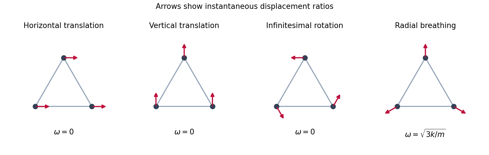
Two translations, an infinitesimal rotation and the radial breathing mode of the equilateral spring triangle
. Details. 
The order of a finite group is its number of elements. Lagrange's theorem states that for a subgroup ,so divides . In particular the order of a group element divides , because it is the order of its generated cyclic subgroup.
For , if some element has order four it generates the whole group, which is therefore the cyclic group . Otherwise every nonidentity element has order two. Choose two distinct ones and put . Cancellation shows , so is the remaining element. Since ,The other products follow: , , and . Thus the second possibility is the Klein four-group. The two groups are not isomorphic because only has an element of order four. This proves the order-four case of the classification of groups of order p squared.
A group homomorphism obeys . It maps identity to identity and inverses to inverses. Its group kernel contains and is closed under , so the subgroup test makes it a subgroup. For and ,Thus ; applying the same argument to gives equality. Hence is a normal subgroup.
Define by . If , then , giving , so this is well-defined. Coset multiplication shows it is a group homomorphism. Its kernel is just the identity coset, since means . It is therefore injective, and the assumed surjectivity of makes it surjective as well. This proves the first isomorphism theorem here:
In the quaternion group, the element commutes with each of , because an element commutes with its square. It then commutes with their negatives too, and with . The set is a subgroup because , and it is central, hence a normal subgroup.
The four quotient cosets are . They square to , and . Reversed products have the same coset: for example , while , so . The same calculation gives and . After signs are identified, these are precisely the products in the Klein four-group. DefineThis preserves all products, is surjective, and has kernel exactly . The first isomorphism theorem therefore givesThis is the quaternion group modulo its centre: the reverse-product relations also show that none of is central, so .
Two elements are conjugate group elements if for some . The conjugacy class of is . Conjugacy is an equivalence relation: it is reflexive using , symmetric by replacing with , and transitive becauseThus the classes partition the group: every element belongs to its own class, and any two classes that intersect are equal. This proves that every element belongs to exactly one class.
If is Abelian, then , so every class is a singleton. In general the elements whose classes are singletons are precisely those commuting with every group element. Thus the center of a group isIt contains . If , then commutes with every , since does and does. The subgroup test therefore proves that is a subgroup. Any two of its elements commute with each other, so it is an abelian subgroup.
For the square centred at the origin with vertices , putThe dihedral group consists of and , . Its eight actions and their matrices areThese exhaust the symmetries: the image of one vertex has four choices and the image of an adjacent vertex has two choices, determining the entire square. For an explicit pair of nonconjugate elements take and . Both have order two, but their determinants are and . A similarity transformation preserves the determinant, so and are not conjugate.
To find the centre, use . A rotation commutes with exactly when , so is even. No reflection commutes with , since while , and . Therefore
A group representation on a vector space is a group homomorphism : and . An invariant subspace obeys for every . A nonzero representation is irreducible if its only invariant subspaces are and . It is a faithful representation if it is injective, equivalently if its group kernel is . Its character is . For inequivalent complex irreducible representations of a finite group, character orthogonality is
Use right-to-left composition of permutations and assign the matrix labels consistently byThe resulting Cayley table, with row multiplying column, isConjugation relabels the entries of a cycle, preserving its length. Thus the conjugacy classes are
Define the permutation representation by , or . Applying it to a basis vector proves . The six assignments above produce exactly the listed matrices. They are distinct, and forces for every , so the representation is faithful.
Every permutation fixes , hence fixes every vector . Therefore is a one-dimensional invariant subspace carrying the trivial representation. Its orthogonal complement issince the inner product with is . Permuting coordinates preserves their sum, so this plane is invariant too. Every real vector has the unique decompositionThus the permutation representation is the direct sum of group representations on the line and the plane.
To find the eigenvectors of , note that . With , its three eigenvalues and eigenspaces areThe only real eigenvalue is one, whose eigenline is , so has no nonzero real eigenvector in . A proper nonzero real invariant subspace of that two-dimensional plane would be a line, giving such an eigenvector. Hence the plane representation is irreducible over .
For the later complex dimension-count theorem one should also establish irreducibility over ; real irreducibility alone would not imply it in general. In the complexified plane, the only candidate -invariant lines are its and eigenlines. But exchanges them:Neither is invariant under the whole group, proving complex irreducibility as well. The required decomposition is thereforewhere is the standard representation of the symmetric group for three letters. Its character is obtained by subtracting one from the number of fixed coordinates: on the three classes it is .
Finally, the sign representation gives a second one-dimensional irreducible, with value on and on the transpositions. These are exactly the two one-dimensional possibilities: if , a one-dimensional representation sends them to commuting nonzero scalars . The relations and imply and . Hence and , the trivial and sign choices. Together with the two-dimensional , these giveThe sum of squares of irreducible representation dimensions leaves room for no other irreducible. Thus there are exactly two one-dimensional and one two-dimensional complex irreducible representations.
Articles by others on the same topic
There are currently no matching articles.