Assume a conventional finite-radius tapping tip whose apex radius and shank are not negligible compared with a trench. The recorded depression is shallower and tip-limited, because the tip contacts the sides before its apex reaches the sharp bottom. Its apparent shape is the accessible envelope of the tip and specimen, not a faithful geometric section.
At a descending edge the separation initially increases, so the oscillation amplitude tends to rise above its setpoint until the controller moves downward. At an ascending edge it tends to fall, until the controller moves upward. For a narrow trench these transients can overlap or partly cancel. With ideal tracking the amplitude remains at its setpoint even when the height is wrong because of tip geometry. Thus a small amplitude error is not proof that the trench bottom was reached.
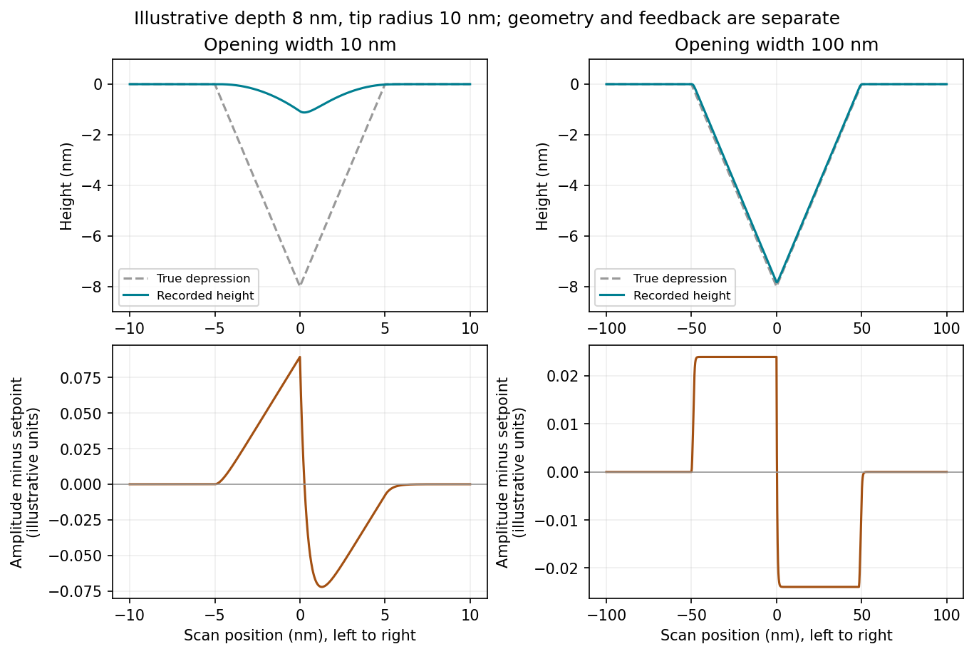
Original illustrative tapping-mode responses to narrow and wide depressions; heights are tip-accessible envelopes and amplitude errors depend on the stated finite-bandwidth model
. Details. 
Width alone does not determine a unique trace: depth, tip radius, cone angle, scan speed and feedback bandwidth are also needed. The plotted traces illustrate the common finite-tip interpretation rather than infer those missing quantities from the drawing.
If the same tip is much smaller than the opening and its shank can enter the depression, the height trace follows the V-shaped depression much more closely, with rounding near the apex and limitations at steep walls. It can reach the actual bottom only if the tip angle and depression depth permit access.
Properly adjusted feedback keeps the measured amplitude close to the setpoint through most of the scan. Small positive and negative amplitude errors occur on descent and ascent with the sign convention in part(a). They are more spatially separated for a wider feature. Reducing scan speed reduces dynamic errors but cannot remove finite-tip exclusion. The figure separates these geometric and feedback effects.
Measure pit dimensions from calibrated height data after background correction, with an explicit pit-boundary convention. Preserve the raw image, lateral calibration and acquisition settings. Level the surrounding terraces and correct line offsets with the pits excluded from the fit; otherwise the deep features bias the background.
Segment each depression relative to its local surface, for example by a reproducible height threshold or a fitted rim. Inspect segmentation overlaid on the image. For noncircular pits, report a metric such as equivalent-area diameteror maximum and minimum caliper diameters, rather than pretending every pit has a circular rim. Apply the same definition to all objects and exclude overlapping or edge-truncated pits where appropriate.
The visible scale bar can calibrate a rendered image approximately, while the original pixel-spacing metadata is preferable. The vertical scale is not a lateral calibration. Estimate uncertainty from pixels, threshold choice, background fits and repeated scans. The tip may be unable to enter narrow pits, so measured depths and diameters require a tip convolution assessment or a sharper calibrated probe. Finally classify populations only against independently validated size/type evidence; the image alone does not establish a universal diameter cutoff for edge, screw and mixed dislocations.
Conductive atomic force microscopy can map current near the pits while recording topography. Use a conducting tip, a suitable counter-contact to the film and an imposed bias, then compare current maps and local current–voltage curves near and away from dislocations. Spreading resistance microscopy is another useful electrical mode when its contact conditions and calibration are suitable.
Current depends on tip contact area, contact resistance, surface oxide, bias and local carrier barriers as well as the material's conductivity. Compare regions under controlled force and bias, check repeated scans for damage and distinguish a geometrical contact artifact from an electrical change. A surface-potential image can complement these measurements, but it does not by itself measure conductivity.
LiftMode is a two-pass measurement separating a measured topographic path from a longer-range interaction measurement. The first pass records height with ordinary topographic feedback. On the second pass the tip retraces that line at a chosen vertical offset above it, reducing contact and short-range contributions while detecting electrostatic or magnetic interactions.
The lift height is relative to the recorded path, not a single constant laboratory height over a corrugated sample. Its usefulness depends on first-pass accuracy and whether the relevant long-range signal remains detectable at that separation.[ref]
Scanning Probe Microscopy Modes by Bruker. LiftMode two-pass description and retracing the stored topography with a height offset
Use Kelvin probe force microscopy to quantify a local contact-potential difference. A conducting tip and sample form a position-dependent capacitor. Apply a voltage with adjustable direct and small alternating components,The electrostatic force is proportional to , so its component at is proportional toup to the chosen force-direction convention. A lock-in amplifier detects this component and a second controller adjusts to null it. At the null, . The compensation voltage becomes the potential image.[ref]
Scanning Probe Microscopy Modes by Bruker. Surface Potential Imaging: conducting probe and electrostatic null measurement
A lift pass can reduce direct topographic interactions. Calibration on a reference with a known work function is required for an absolute work-function interpretation, and the sign convention must state which electrode is biased. On a semiconductor the result can include surface band bending, trapped charge and surface chemistry, so it need not equal a simple map of bulk electrochemical potential.
The measured potential is a spatially weighted electrostatic signal, not an infinitesimal-point voltage. The apex, cone and cantilever all contribute capacitance; increasing lift height weakens the signal and broadens its lateral averaging. Small pits can consequently show reduced or distorted contrast.
Imperfect topographic tracking changes the true separation on the lift pass, producing crosstalk correlated with pit geometry. Tip contamination or work-function drift changes the reference. Adsorbed water, mobile charges, illumination, atmosphere and surface states can change the specimen during measurement; semiconductor band bending can also depend on the applied electrical excitation.
There is a tradeoff between small lift height and suppressing short-range/topographic interference. Repeat at several heights, check trace/retrace and an electrical reference, and compare with independently measured electrical response. A stable potential contrast is evidence of a local electrostatic difference, not by itself proof of a particular dislocation's conductivity.
Articles by others on the same topic
There are currently no matching articles.