The map shows Coulomb blockade with discrete single-electron charging: low-current diamonds separate charge-stable regions from finite-bias transport windows. A small conducting island or quantum dot must be tunnel-coupled to source and drain, with a gate shifting its electrochemical potential. Charging prevents sequential transport until an island addition/removal energy enters the bias voltage window.
The tunnel resistances should substantially exceed the resistance quantum , preventing charge fluctuations from washing out integer island occupancy, while still permitting a measurable current. Temperature and tunnel broadening must be small compared with the addition-energy scale. Here the smaller diamonds imply , so , or ; resolving the inferred 1 meV orbital structure requires the stricter scale . Stray capacitance and unintended multiple islands can complicate this simple interpretation.
Assume the usual one-lead-biased measurement, with drain grounded and the gate referred to that ground; the printed map does not separately specify the wiring. This assumption is needed to assign individual source/drain capacitances. In this Coulomb diamond capacitance extraction, the smaller zero-bias gate intervals are 5 mV wide. In the constant interaction model with no orbital gap between those additions,An upper diamond tip lies at gate 123.75 mV between the zero-bias vertices 120 and 125 mV and at bias 2.50 mV. Its positive and negative edge slopes are therefore and . Reservoir alignment givesThe gate capacitance is not negligible in the second denominator. ConsequentlyThe consistency check is , matching the smaller tip's bias energy. The conventional electrostatic charging energy is 1.25 meV; it is half the charging energy contribution to the addition energy. A different applied-bias convention changes the slope formulas, so the convention must accompany the extraction.
The addition energy has both charging and orbital terms,The larger diamonds indicate quantum dot shell closure after 2, 6 and 12 electrons. A two-dimensional isotropic harmonic oscillator confinement, , explains that sequence: shell has orbital states and capacity after spin degeneracy. The cumulative capacities are . Within a degenerate shell, the extra orbital term vanishes to this approximation; crossing a shell boundary costs an extra .
The gate capacitance lever arm is . Large and small gate widths differ by , so . Equivalently the tip energies differ by . Confinement anisotropy, exchange and disorder would split the ideal degeneracies; the diagram supports approximate shell symmetry rather than proving a perfectly parabolic potential.
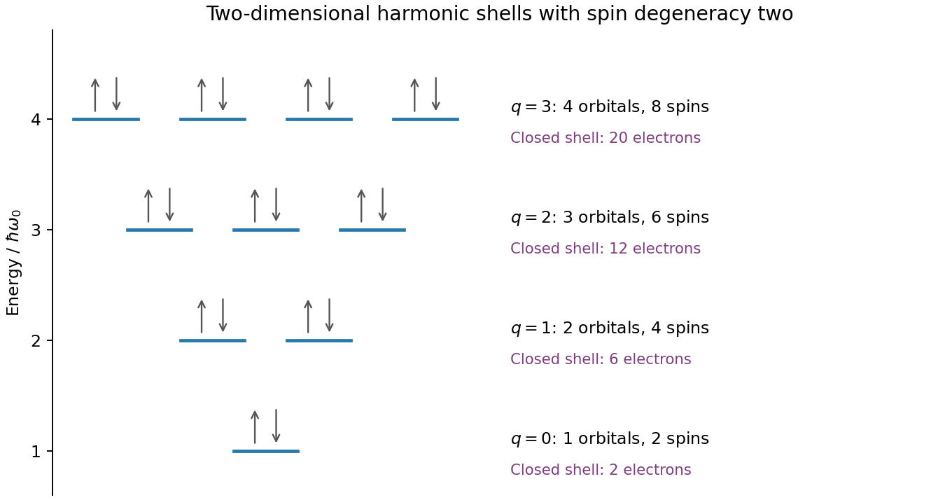
Original spin-degenerate two-dimensional oscillator shell capacities and closed-shell electron counts
. Details. 
For an isolated easy-axis ferromagnet undergoing coherent reversal, the ideal low-temperature loop is approximately rectangular, switching between at . It has remanent Magnetization and a large response near switching. An ideal compensated antiferromagnet has essentially no remanence and a small, approximately reversible linear net Magnetization at fields far below its exchange/spin-flop scales. Strong antiferromagnetic exchange makes substantial canting costly, so its low-field magnetic susceptibility is small relative to the ferromagnet's unsaturated switching response.
This comparison does not say the ferromagnet has a larger differential slope at every field: on its saturated branches can also be small. Nor does it rule out spin-flop transitions at much larger fields, outside the sketched range. The original plot uses arbitrary normalized scales.
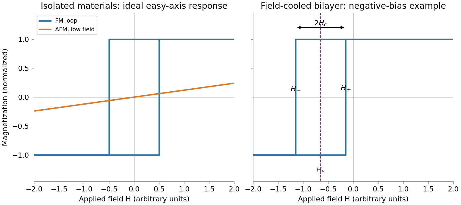
Original isolated-ferromagnet and antiferromagnet responses, and a field-cooled shifted bilayer loop
. Details. 
Heat the bilayer into a window , apply an in-plane magnetic field sufficient to align the ferromagnet, and cool through the antiferromagnet's ordering/blocking range while retaining the field. The ferromagnet supplies a preferred interfacial spin direction as the antiferromagnet orders. Sufficient antiferromagnetic anisotropy then pins part of the interfacial spin configuration, producing unidirectional magnetic anisotropy rather than merely uniaxial magnetic anisotropy in the ferromagnet.
Measure a full major hysteresis loop after removing the cooling field, and compare with the isolated ferromagnet, a zero-field-cooled bilayer and the result of reversing the cooling-field direction. Those controls separate a true loop-centre shift from a changed coercive width, minor-loop artefacts or trapped applied field. The effect requires appropriate interfacial exchange and stable pinning; an ideally compensated or freely rotating interface need not produce a large bias. Exchange anisotropy in coupled ferromagnetic/antiferromagnetic material was demonstrated in the classic experiment below.[ref]
New Magnetic Anisotropy by W. H. Meiklejohn and C. P. Bean. Physical Review 102 (1956), pp. 1413–1414
Write the descending and ascending switching fields as and . The exchange bias loop centre and magnetic coercivity half-width areWith exchange bias, a field-cooled bilayer has , often a shift opposite to the cooling field for the conventional negative-bias case shown in the diagram. The sign is not universal; it depends on interfacial coupling and preparation. A simple rigid-pinning estimate is .
Cooling farther below the blocking range usually strengthens antiferromagnetic anisotropy and suppresses thermal relaxation, so the magnitude of the shift and often the coercive width grow. Close to or above the blocking temperature the shift disappears; the blocking temperature can be below . Repeated cycling can rearrange interfacial spins and reduce the bias, and the two reversal branches can acquire different shapes. Thus increasing low-temperature asymmetry is a common tendency, not a guaranteed monotonic law for every interface.
Articles by others on the same topic
There are currently no matching articles.