Original archive: Cambridge FOI 2024/50 released ZIP. The original is the member
NanoMPhil Paper 2 2021.pdf, physical pages 1–13.Rolling graphene into a single-walled carbon nanotube quantizes the circumferential wave vector, leaving a set of one-dimensional longitudinal subbands. At each subband edge the group velocity tends to zero, producing a Van Hove singularity in the density of states. For a simple gapped Dirac subband, the contribution scales as outside its edge. At low temperature the valence states below the Fermi level are occupied and the conduction states above it are empty. A semiconducting tube has a gap; an ideal metallic tube has gapless channels as well as higher-subband singularities.
For light polarized along the tube, the strongest allowed interband transitions connect corresponding subbands while approximately conserving axial wave vector and circumferential angular momentum. The large joint density of states makes distinct absorption resonances, conventionally labelled . Strong electron–hole interactions produce bound excitons, so the observed optical resonances differ from the noninteracting band separations. Defects, doping, bundling and dielectric screening change peak energies and oscillator strengths. The original schematic below depicts the subband-edge structure, not measured spectra.
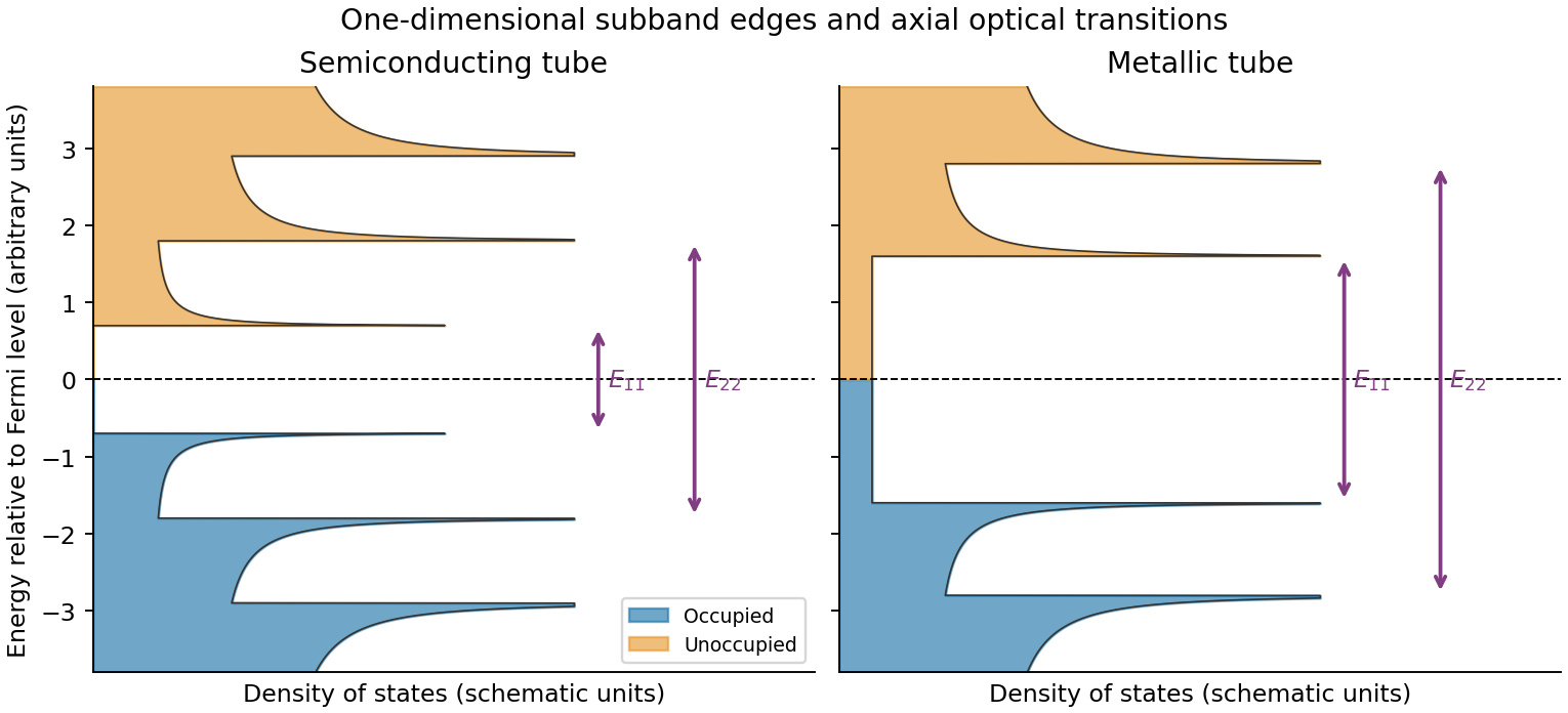
Original schematic occupied and unoccupied nanotube densities of states and allowed optical transitions
. Details. With the graphene lattice-vector length , the carbon nanotube chiral vector is . The vectors meet at , givingHere is circumference, diameter, and the carbon nanotube chiral angle is measured from the zigzag direction. Nanotube zone folding gives a nominal metallic tube when and a semiconducting tube otherwise. Evaluating all the supplied indices gives the following derived results:All eleven listed tubes are semiconducting in the zone-folding classification. Curvature can open small gaps in some nominally metallic non-armchair tubes, but none of these indices falls in that nominal metallic class.
Diameter gives a useful inverse-size trend in transition energies, and the full chiral indices constrain the electronic band structure much more strongly. They do not by themselves give the perceived solution colour through a simple geometrical rule: one needs the visible absorption spectrum, transition strengths and widths, exciton/environment shifts, concentration, optical path and illumination. The observed transmitted colour is complementary to the absorbed spectrum, not a direct label for the band gap. Structure-assigned excitation–emission measurements provide an experimental connection between chiral structure and optical transitions.[ref]
Structure-assigned optical spectra of single-walled carbon nanotubes by Sergei M. Bachilo and others. Science 298 (2002), pp. 2361–2366, structure assignment of semiconducting-tube optical transitions
One application is a semiconducting nanotube transistor array. Removing metallic tubes prevents conducting bridges that would bypass gate control; a narrow chirality distribution also narrows the spread of band gaps and switching behaviour. High charge carrier mobility and thin flexible channels are attractive, but contact resistance, tube alignment, residual metallic contamination, dielectric traps and the cost/yield of sorting still limit uniform large-area circuits.
A second is a wavelength-selective near-infrared photodetector or emitter. A selected chirality concentrates absorption and emission around its characteristic nanotube optical transitions, avoiding the broad mixed-tube response. Optical selectivity can be tailored by choosing the species. Limitations include low absolute emission yield, dark exciton states, contact-related recombination, environmental spectral shifts and quenching by bundles or metallic contaminants. Optical and electrical characterization after device processing is needed; the sorting label alone does not guarantee device performance.
Prepare size-characterized gold-particle ensembles, heat them on a calibrated in-situ electron diffraction stage, and follow the loss of sharp fcc diffraction features and appearance of liquid-like diffuse scattering. Measure the particle size distribution rather than treating a polydisperse ensemble as one diameter. Temperature-dependent weakening of a diffraction peak alone is insufficient: thermal vibrations, particle motion, coalescence, evaporation and beam damage can also reduce intensity. Low-dose repeats, heating/cooling runs, size checks before and after heating, a bulk-like reference and support-dependent controls help distinguish melting from those effects. Electron diffraction measurements on gold particles down to about 2 nm are a classic demonstration.[ref]
Size effect on the melting temperature of gold particles by Ph. Buffat and J-P. Borel. Physical Review A 13 (1976), pp. 2287–2298, abstract: scanning diffraction and size-distribution analysis
The physical origin is the large interface contribution to free energy at small radius. A curved solid–liquid interface raises the solid's thermodynamic equilibrium chemical potential relative to the flat-interface case, so coexistence occurs below the bulk melting temperature. Reduced coordination and surface disorder provide a microscopic interpretation, but the quantitative continuum relation is a free energy balance, not simply a claim that every surface atom has a universal lower melting point.
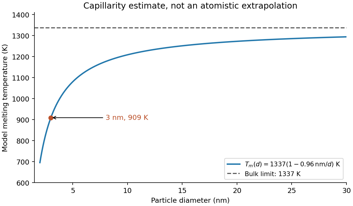
Let be the liquid-minus-solid free energy density at the same temperature. Near the bulk coexistence temperature , linearization givesFor a sphere, an interface displacement changes area and volume with . Equality of the bulk driving force and the capillary cost at a curved solid–liquid interface therefore gives . Equivalently, differentiating gives the same stationary radius. Combining the expressions yieldsThis form of the Gibbs-Thomson effect assumes isotropic interfacial energy, a spherical interface, bulk-like latent heat per volume and a near-coexistence free energy expansion. More detailed free-particle models must distinguish solid–vapor, liquid–vapor and solid–liquid energies.
The radius is half the diameter, , and the latent heat density is . HenceUsing the diameter directly in the radius formula would underestimate the depression by a factor of two. The result is the stipulated continuum-model estimate; at only a few nanometres atomistic structure and support effects can matter substantially.
In terms of diameter , the model isThus melting temperature rises toward the bulk value as diameter increases, with a depression proportional to . The analytic sketch below includes the calculated point. It deliberately does not extrapolate the continuum expression down to a zero or negative melting temperature.
Facet-dependent energies, non-spherical shapes, size-dependent interfacial energies and latent heat, structural changes or magic cluster sizes can modify the trend. Premelting can broaden the transition. A substrate or encapsulating matrix changes interface energetics and can stabilize or destabilize the solid. Ligands, impurities, strain, particle size distributions, coalescence during heating and nonequilibrium temperature/beam effects can shift the measured transition. These possibilities motivate separate thermal, structural and size controls rather than a fit to diameter alone.


The map shows Coulomb blockade with discrete single-electron charging: low-current diamonds separate charge-stable regions from finite-bias transport windows. A small conducting island or quantum dot must be tunnel-coupled to source and drain, with a gate shifting its electrochemical potential. Charging prevents sequential transport until an island addition/removal energy enters the bias voltage window.
The tunnel resistances should substantially exceed the resistance quantum , preventing charge fluctuations from washing out integer island occupancy, while still permitting a measurable current. Temperature and tunnel broadening must be small compared with the addition-energy scale. Here the smaller diamonds imply , so , or ; resolving the inferred 1 meV orbital structure requires the stricter scale . Stray capacitance and unintended multiple islands can complicate this simple interpretation.
Assume the usual one-lead-biased measurement, with drain grounded and the gate referred to that ground; the printed map does not separately specify the wiring. This assumption is needed to assign individual source/drain capacitances. In this Coulomb diamond capacitance extraction, the smaller zero-bias gate intervals are 5 mV wide. In the constant interaction model with no orbital gap between those additions,An upper diamond tip lies at gate 123.75 mV between the zero-bias vertices 120 and 125 mV and at bias 2.50 mV. Its positive and negative edge slopes are therefore and . Reservoir alignment givesThe gate capacitance is not negligible in the second denominator. ConsequentlyThe consistency check is , matching the smaller tip's bias energy. The conventional electrostatic charging energy is 1.25 meV; it is half the charging energy contribution to the addition energy. A different applied-bias convention changes the slope formulas, so the convention must accompany the extraction.
The addition energy has both charging and orbital terms,The larger diamonds indicate quantum dot shell closure after 2, 6 and 12 electrons. A two-dimensional isotropic harmonic oscillator confinement, , explains that sequence: shell has orbital states and capacity after spin degeneracy. The cumulative capacities are . Within a degenerate shell, the extra orbital term vanishes to this approximation; crossing a shell boundary costs an extra .
The gate capacitance lever arm is . Large and small gate widths differ by , so . Equivalently the tip energies differ by . Confinement anisotropy, exchange and disorder would split the ideal degeneracies; the diagram supports approximate shell symmetry rather than proving a perfectly parabolic potential.
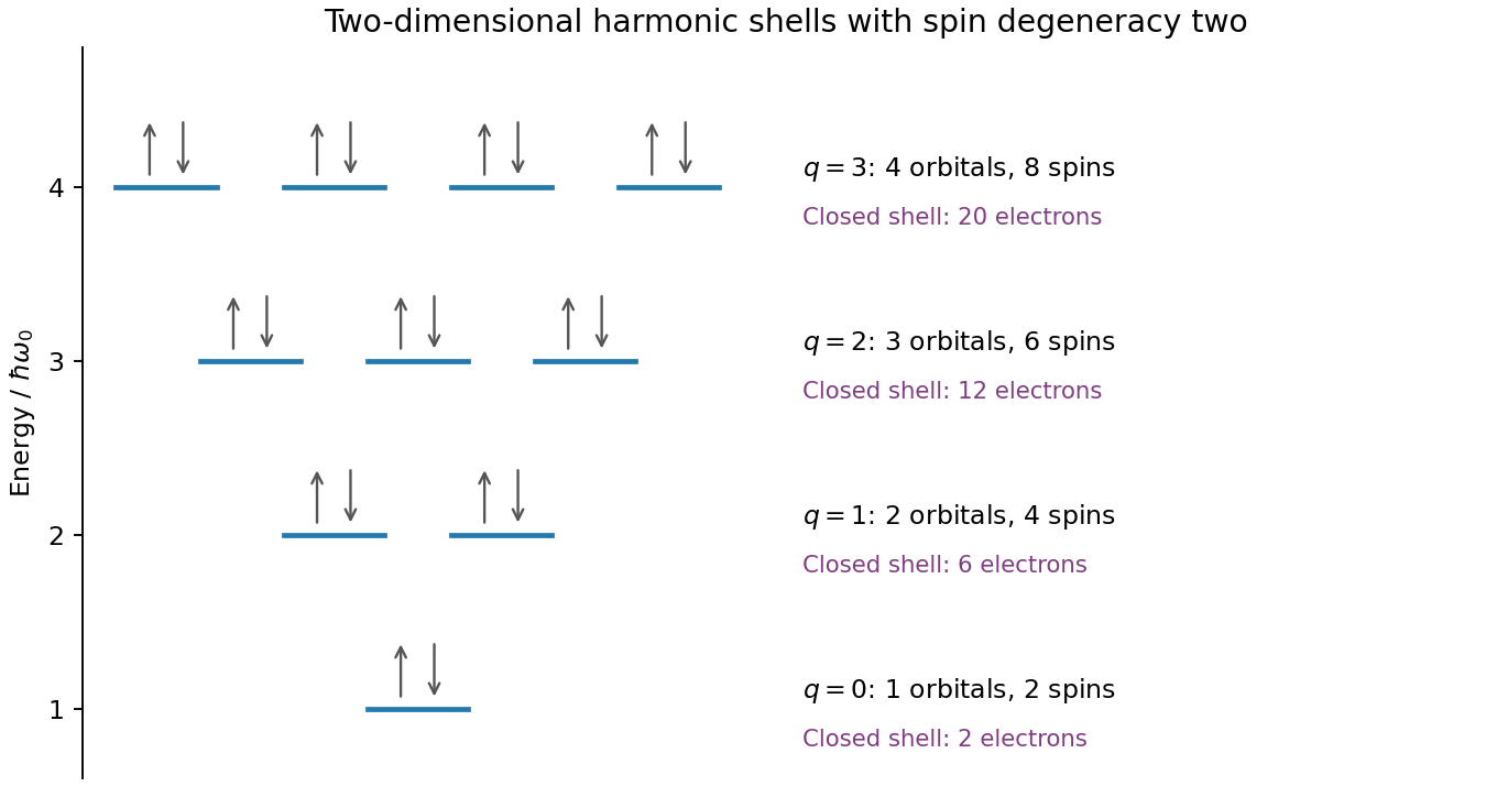
Original spin-degenerate two-dimensional oscillator shell capacities and closed-shell electron counts
. Details. 
For an isolated easy-axis ferromagnet undergoing coherent reversal, the ideal low-temperature loop is approximately rectangular, switching between at . It has remanent Magnetization and a large response near switching. An ideal compensated antiferromagnet has essentially no remanence and a small, approximately reversible linear net Magnetization at fields far below its exchange/spin-flop scales. Strong antiferromagnetic exchange makes substantial canting costly, so its low-field magnetic susceptibility is small relative to the ferromagnet's unsaturated switching response.
This comparison does not say the ferromagnet has a larger differential slope at every field: on its saturated branches can also be small. Nor does it rule out spin-flop transitions at much larger fields, outside the sketched range. The original plot uses arbitrary normalized scales.
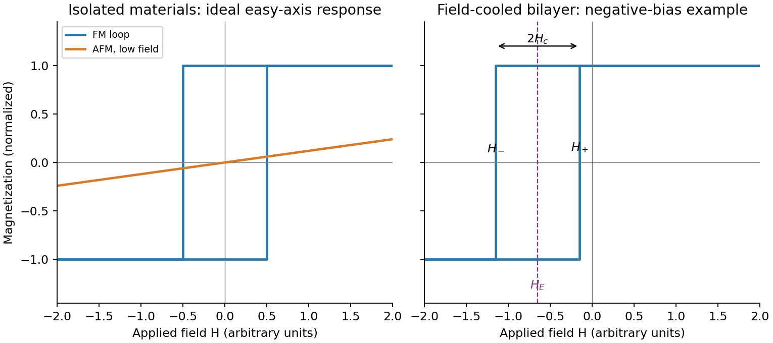
Original isolated-ferromagnet and antiferromagnet responses, and a field-cooled shifted bilayer loop
. Details. 
Heat the bilayer into a window , apply an in-plane magnetic field sufficient to align the ferromagnet, and cool through the antiferromagnet's ordering/blocking range while retaining the field. The ferromagnet supplies a preferred interfacial spin direction as the antiferromagnet orders. Sufficient antiferromagnetic anisotropy then pins part of the interfacial spin configuration, producing unidirectional magnetic anisotropy rather than merely uniaxial magnetic anisotropy in the ferromagnet.
Measure a full major hysteresis loop after removing the cooling field, and compare with the isolated ferromagnet, a zero-field-cooled bilayer and the result of reversing the cooling-field direction. Those controls separate a true loop-centre shift from a changed coercive width, minor-loop artefacts or trapped applied field. The effect requires appropriate interfacial exchange and stable pinning; an ideally compensated or freely rotating interface need not produce a large bias. Exchange anisotropy in coupled ferromagnetic/antiferromagnetic material was demonstrated in the classic experiment below.[ref]
New Magnetic Anisotropy by W. H. Meiklejohn and C. P. Bean. Physical Review 102 (1956), pp. 1413–1414
Write the descending and ascending switching fields as and . The exchange bias loop centre and magnetic coercivity half-width areWith exchange bias, a field-cooled bilayer has , often a shift opposite to the cooling field for the conventional negative-bias case shown in the diagram. The sign is not universal; it depends on interfacial coupling and preparation. A simple rigid-pinning estimate is .
Cooling farther below the blocking range usually strengthens antiferromagnetic anisotropy and suppresses thermal relaxation, so the magnitude of the shift and often the coercive width grow. Close to or above the blocking temperature the shift disappears; the blocking temperature can be below . Repeated cycling can rearrange interfacial spins and reduce the bias, and the two reversal branches can acquire different shapes. Thus increasing low-temperature asymmetry is a common tendency, not a guaranteed monotonic law for every interface.
For this self-assembly into a colloidal crystal, four useful elements are building blocks, interactions, environment and reversible dynamics. The building blocks here are nearly monodisperse polymer spheres; their shape and size distribution constrain the accessible packing. Their interactions include excluded volume, Van der Waals forces and electrostatic or steric stabilization, which set the free energy landscape. The aqueous environment supplies temperature, viscosity, ionic strength, confinement and concentration controls. Finally, Brownian motion and rotation must let particles encounter one another and rearrange or detach from incorrect contacts. Attractions that bind every collision irreversibly favour an amorphous aggregate rather than an annealed colloidal crystal. These four categories include both thermodynamic selection and the transport/kinetic access needed to realize it.
A useful microscopic screening estimate compares thermal energy with the buoyant gravitational potential energy over one particle radius. Write and . The sedimentation length is , and the gravitational Peclet number isUsing and requiring givesEquivalently, combining Stokes law speed and diffusion coefficient gives . Buoyancy, not the full polystyrene density, is essential to the estimate. Taking a diameter rather than radius as the comparison length changes the numerical cutoff by an order-one factor.
There is no universal largest particle that stays uniformly suspended indefinitely. If uniformity over a vessel height is required, use , not merely . For example gives a much smaller radius, about 58 nm. Observation time, density matching, convection, particle polydispersity and shape also matter. Independent of sedimentation, electrostatic/steric barriers must prevent aggregation; low ionic strength, suitable surface chemistry and clean solvent can be as important as size.
Increase particle volume fraction slowly by controlled evaporation or gentle concentration until ordering becomes favourable, while preserving sufficient colloidal repulsion to prevent irreversible sticking. Hard-sphere-like monodisperse suspensions can crystallize by packing entropy; weak, reversible attractions can also favour ordered assembly if they allow defect correction. A controlled drying front or patterned surface may guide the orientation, and gentle sedimentation can create a concentration gradient that crosses the ordering range.
The practical requirement is slow structural change relative to Brownian motion, with uniform temperature, well-characterized ionic strength and a narrow size distribution. An abrupt salt addition or rapid drying can remove the repulsive barrier and trap aggregates instead of growing a crystal. Scattering or microscopy should distinguish crystalline peaks/order from merely increased turbidity.
Flocculation indicates that the attraction/kinetic balance has changed: electrolyte may screen a double-layer barrier; pH may reduce surface charge; multivalent ions can promote aggregation; added polymer can bridge particles or cause depletion force; poor solvent conditions can collapse stabilizing layers. Rapid evaporation concentrates both particles and salts and can force contacts faster than they anneal. Aggregates then sediment much faster because their effective buoyant size has grown.
Check ionic strength, pH, surface charge and the particle size distribution before and during assembly. Dialyse or reduce salt where appropriate, restore surface charge, add a nonbridging steric stabilization with a compatible solvent, and slow the concentration step. Compare untreated and deliberately salt-screened controls. Restoring repulsion after irreversible aggregation may not redisperse the particles, so prevention is preferable to assuming all settled material can be recovered.
Three suitable examples are cubes bounded mainly by facets, octahedra bounded by facets, and truncated octahedra bounded by both and facets. These are crystallographically distinct shapes rather than three arbitrary rounded particle outlines.
At fixed volume the thermodynamic equilibrium shape minimizes , with an edge/corner correction when particles are very small. In the Wulff construction, facet support-plane distances scale as their interfacial free energies. Silver's clean low-index energies, selective adsorption of ligands or ions, solvent chemical potential and possible support contact alter those energies. Crystal twinning and elastic strain can add further costs or stabilize multiply twinned forms. A face with slow attachment kinetics can also survive during growth even when that morphology is not the thermodynamic equilibrium Wulff shape. Homogeneous nucleation describes where nuclei form; it does not guarantee an thermodynamic equilibrium final shape.
In a polyol process, a hot polyol such as ethylene glycol acts as solvent and reductant for a silver precursor. Nucleation creates seeds; controlled reduction supplies atoms for their subsequent growth, while polyvinylpyrrolidone adsorption and seed crystal twinning favour anisotropic growth. For the common silver nanowire route, a fivefold-twinned seed can develop into a pentagonal wire with predominantly side faces and growth at less-passivated ends. Cross-sectional microscopy and diffraction of microtomed wires provide evidence for that twinned structure rather than an inference from a long outline alone.[ref]
Polyol Synthesis of Uniform Silver Nanowires: A Plausible Growth Mechanism and the Supporting Evidence by Yugang Sun and others. Nano Letters 3 (2003), pp. 955–960, pentagonal cross sections and fivefold twinning
The aspect ratio depends on seed population and twin survival, relative end/side growth rates, precursor feed and reduction rate, PVP coverage, temperature, trace halides, dissolved oxygen and growth time. High aspect ratio requires a suitable population of twinned seeds, suppression of competing particle nucleation and continued atom supply while sidewall thickening is restrained. These variables must be controlled together; adding more capping polymer alone is not a universal recipe. Advantages are solution processing, substantial yield and tunable dimensions without an etched hard template. Disadvantages include sensitive batch reproducibility, particle by-products, residual insulating ligand, purification, oxidation/tarnish and nanowire junction resistance in later films. Compare seed/capping/halide controls using microscopy and size distributions, not only solution colour.
A transparent metallic network must span the patterned electrode with many redundant current paths while obscuring little area. For random rods, number density times squared wire length is a useful percolation measure; greater aspect ratio generally reaches a connected network at lower coverage. Conductivity also depends on intrinsic metal resistivity, wire cross section, orientation, length distribution, wire–wire contact resistance and the number of junctions along each spanning path. Insulating capping layers can make nanowire junction resistance dominate even when the individual wires are excellent conductors.
Near the connectivity threshold, small density changes or wire breaks produce large resistance changes. For a narrow stripe, finite-size effects and orientation matter: a macroscopic sheet-average percolation result does not ensure a reliable 100 µm-wide path. Optical performance depends on coverage, metal extinction, wire diameter, aggregation, optical haze, substrate transmission and any binder. Increasing wire density lowers resistance but usually lowers transmission. Welding, pressing or suitable embedding can improve contacts with less additional optical coverage than simply adding metal.[ref]
Self-limited plasmonic welding of silver nanowire junctions by Erik C. Garnett and others. Nature Materials 11 (2012), pp. 241–249, junction-localized welding mechanism
The stripe has squares, so its end-to-end resistance is ; the stated sheet-resistance limit requires a stripe resistance below 5 kΩ, not 20 Ω. The sketch below separates sparse connectivity, redundant paths and junction quality.
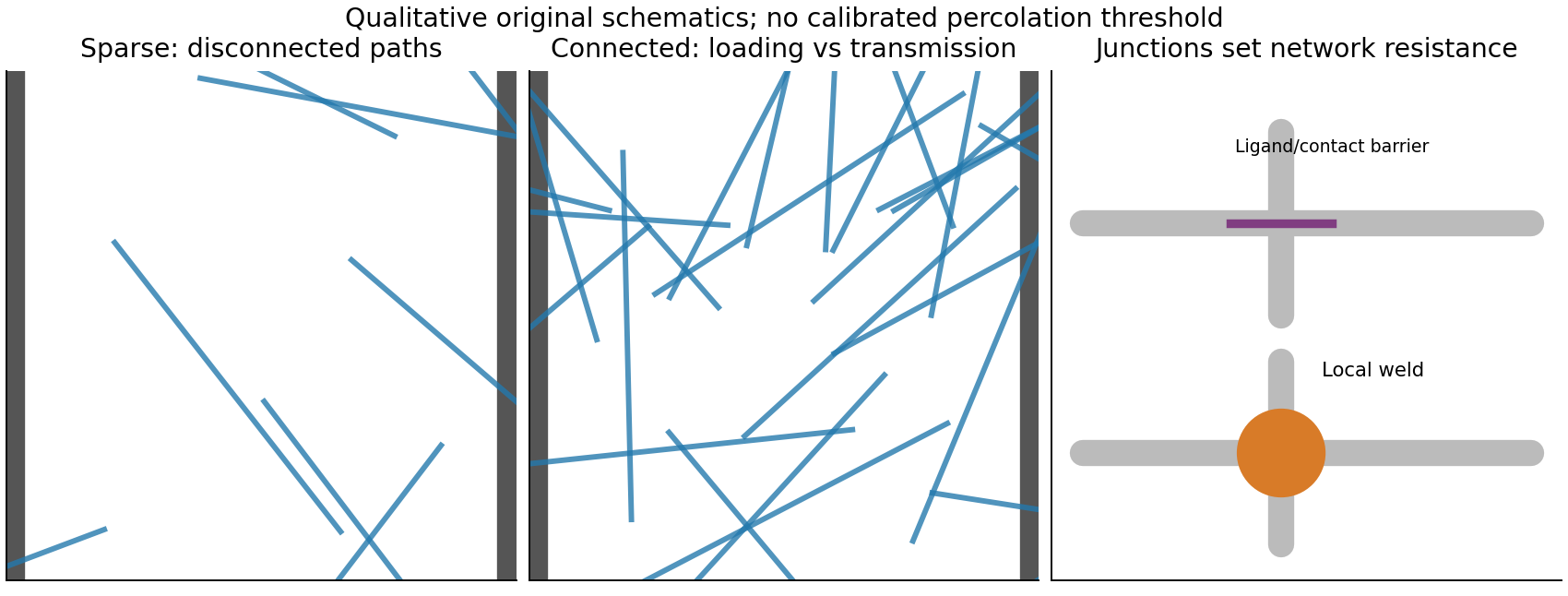
Original network schematics distinguishing connectivity, optical coverage and wire-junction resistance
. Details. 
Three credible architectures are a welded silver nanowire network; a thin silver nanowire network with a conducting polymer overcoat; and a nanocrystalline silver grid formed from nanoparticle ink. Silver provides low intrinsic resistivity. A sparse long-wire network can be both flexible and highly transmitting if its junctions are well connected. A thin, optically weak conducting polymer overcoat can bridge junctions and smooth the surface, provided its added absorption and moisture sensitivity are controlled. A fine grid offers a more directly designed optical/electrical trade-off and does not rely on operating near random percolation.
For a quantitative grid feasibility screen, take pitch , line width and metal thickness . An opaque-line square-grid estimate gives . With a transmitting polymer substrate of 0.95, the combined estimate is 0.912. The sheet resistance is approximately . Even an effective silver resistivity four times gives , with a coating thinner than 400 nm. There are about 20 mesh periods across the stripe, making the finite-width design more credible than a pitch comparable with its whole width.
These are feasible material/process choices, not guaranteed specifications for every film carrying those names. For the two nanowire architectures, choose wire dimensions, loading and junction treatment to pass the same finished-stripe measurements; the hybrid's optical budget must include its overcoat. Measure transmission at 550 nm with its reference stated, sheet resistance, profile thickness, bend-cycle stability and pattern continuity. Bare nanotube or graphene networks should not be assumed to meet this demanding resistance–transmission combination without additional metallic conduction or other demonstrated improvement.
For the silver nanowire network, synthesize or source long, narrow wires, remove excess ligand without causing aggregation, formulate a stable coating ink and coat the flexible web by a scalable method such as slot-die coating or gravure printing. Dry below the substrate's damage temperature, then press or locally weld junctions and embed or cap the network if required. Define 100 µm stripes by masked coating, a printing-compatible patterned wetting layer, or post-coating laser ablation; provide robust end contacts and remove stray bridges between adjacent stripes. Roll processing offers throughput, but coffee-ring effect, wire alignment, random weak links and ablation damage require inline optical/electrical inspection. Verify that the local junction treatment improves resistance without simply darkening the whole film.
For the silver nanoparticle-derived grid, use a repeatable nanoimprint lithography to form a fine mesh inside the outer 25 mm by 100 µm stripe pattern. Fill the channels with a silver nanoparticle ink, remove excess from the transparent openings, and consolidate the metal by substrate-compatible chemical, photonic or low-temperature thermal sintering. Transfer or embed the grid into the polymer surface and add electrical pads. The quantitative design in part (b) sets target pitch, line width and thickness; the large-scale process must maintain those dimensions and a continuous metal cross section. A master enables repeated replication and deterministic open area, but tooling cost, incomplete filling, residual metal in windows, shrinkage cracks, imperfect sintering and adhesion are important limitations. Test the finished patterned stripes, rather than relying on a large unpatterned test coupon alone.
A two-dimensional electron gas is confined into discrete subbands perpendicular to an interface while retaining nearly free motion in its plane. It is not a literal zero-thickness electron sheet. In a GaAs/AlGaAs semiconductor heterostructure, the band offset and self-consistent band bending confine electrons on the GaAs side. Donors in AlGaAs can supply electrons while an undoped spacer separates them from the ionized dopants, reducing impurity scattering. This modulation-doping arrangement yields a high-mobility channel, with the lowest confinement subband occupied when the confinement spacing exceeds the Fermi and thermal scales. Gates tune the density or locally deplete the channel into constrictions. Low-temperature Hall and longitudinal measurements test the resulting sheet density and transport quality.
Use the magnitudes of the single-electron-band Drude Hall relation and longitudinal sheet resistivity:The given values are two-dimensional resistivities, so no sample thickness is inserted. ThusThe carrier sign follows from a specified Hall-voltage orientation; these calculations use positive magnitudes. A parallel conducting layer, several occupied subbands or a quantized Hall plateau would require a different interpretation of a single-field measurement.
For a parabolic two-dimensional electron gas with one valley and two spin states, the density of states per area is . Integrating from the subband edge to the zero-temperature Fermi energy gives , henceHere , and the energy is measured from the occupied subband bottom. Equivalently . ThereforeThe spin factor is already included in ; counting it again would halve the energy incorrectly.
This is transverse magnetic focusing. The depleted gates form reflecting boundaries and two constrictions. A narrow quantum point contact collimates carriers into cyclotron trajectories with cyclotron radius . When an integer number of semicircular skipping arcs links the two openings, the collector couples particularly strongly to the injector population. A floating voltage contact then changes its electrochemical potential to satisfy zero net current, producing a peak in the measured nonlocal voltage. Sweeping the field changes the arc diameter, moving the focused population into or away from the collector.
The connection condition is for integer , with the higher orders requiring specular reflections. The effect needs ballistic electron transport, sufficiently narrow openings and a smooth boundary. Electron phase coherence can add interference structure, but the basic geometrical focusing condition is semiclassical.[ref]
Coherent electron focusing with quantum point contacts in a two-dimensional electron gas by H. van Houten and others. Physical Review B 39 (1989), pp. 8556–8575, focusing geometry and peak structure
There is a polarity qualification in the printed geometry. The electron charge is negative: for a field out of the page, an electron launched upward through the left opening bends left, not toward the right opening. A direct left-opening-to-right-opening focusing path in the upper region therefore requires the field into the page; the printed outward field supports the reverse connection. Reversing conventional current reverses the occupation perturbation and voltage sign, but does not reverse the curvature of an individual electron. Thus the standard injector-to-collector explanation describes the focusing mechanism, while the asserted signed voltage increase requires a consistent field/lead convention. The calculated results below are peak-field magnitudes; taking outward field positive gives negative fields for direct left-to-right electron injection.
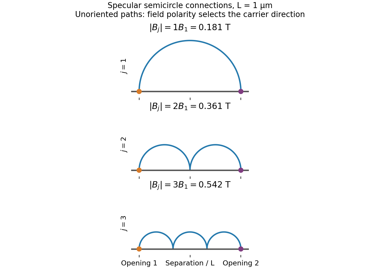
Original semicircular connections for three focusing orders; trajectories are shown without carrier-direction arrows
. Details. 
Substituting into givesUsing the density-derived Fermi wave vector gives the first three peak magnitudesThe equally spaced sequence follows from the number of reflected half-orbits, not from successive quantum Hall fillings. The field polarity selecting a given injector–collector orientation follows from the Lorentz force direction.
The transport mean free path is , while . Eliminating the scattering time gives . The usual ballistic focusing mobility criterion therefore givesA more geometrically faithful first-peak survival criterion uses the semicircular path length , giving . There is no sharp universal visibility threshold: clearly resolved peaks favour , small aperture broadening and specular reflection. The mobility inferred in part (ii) corresponds to , comfortably above both estimates. Higher-order peaks can still be reduced by boundary roughness even when bulk mobility is high.
Treat the top gate as a parallel-plate capacitor, neglecting fringing and assuming its voltage change couples to the 2DEG without a dominant trap or series-capacitance correction. Its capacitance per area and induced electron density areIn this top-gate density tuning, a positive gate change increases the electron density in this model, giving . Since ,The fields rise by a factor , not by the density ratio itself. Finite quantum capacitance is a small correction here: the one-subband value is much larger than the stated geometric capacitance per area.
The highest-field plateau is labelled , so it is the plateau in the filling factor, with the longitudinal resistivity returning to approximately zero after the transition near 10 T. The odd integer indicates a resolved spin branch at these fields; assuming a permanent twofold spin degeneracy for every orbital Landau level would misidentify the plotted sequence.
For a nominal exactly filled state at a chosen field , the density target is . Combining this with the same gate capacitor model gives the required gate-voltage change relative to the original ungated-density reference:Taking as the graph's onset-scale estimate gives andRelative to the positive 0.2 V setting in part (v), this is an additional change of approximately . An absolute laboratory gate voltage cannot be obtained without its initial offset or threshold; the calculated quantities are voltage changes.
There is a graphical/model qualification: a quantum Hall plateau occupies a finite field interval, and its onset is not an exact statement that at that edge. The plot identifies from about 10 T onward but does not specify a unique plateau-centre field or the gate setting at which the trace was recorded. The boxed formula gives the result for any selected target field. For comparison, the nominal exact-filling fields are 12.39 T at the original density and 18.34 T at the unchanged positive 0.2 V density. Thus the graph must not be combined silently with the latter density as if its onset uniquely fixed the same gate bias.
Brownian motion is the irregular thermal displacement produced by fluctuating molecular forces from the surrounding liquid. In the overdamped regime its long-time displacement is diffusive, with mean squared displacement proportional to time. It brings nanoscale building blocks into contact and lets them sample orientations and escape weak incorrect contacts. Interparticle forces bias this exploration toward lower-free-energy structures; thermal motion alone does not select a particular crystal. Strong irreversible attraction, high viscosity or glassy arrest can stop the defect correction needed for successful self-assembly.
Articles were limited to the first 100 out of 112 total.
Articles by others on the same topic
There are currently no matching articles.