The five tasks below concern a scanned Michelson interferometer. The original dashed curves are labelled visibility in arbitrary units; divide them by their maximum to obtain normalized interferometric visibility, which lies between zero and one.
A non-polarizing beam splitter divides the incident spectrum into a fixed arm and an arm with a translating mirror. Recombining their returned fields gives a detector signal as a function of mirror position . The round-trip optical path difference is relative to the equal-arm position, so the delay is in air approximated as vacuum. Record both detector signal and calibrated position, subtract the constant background, and take a Fourier transform of the interferogram.
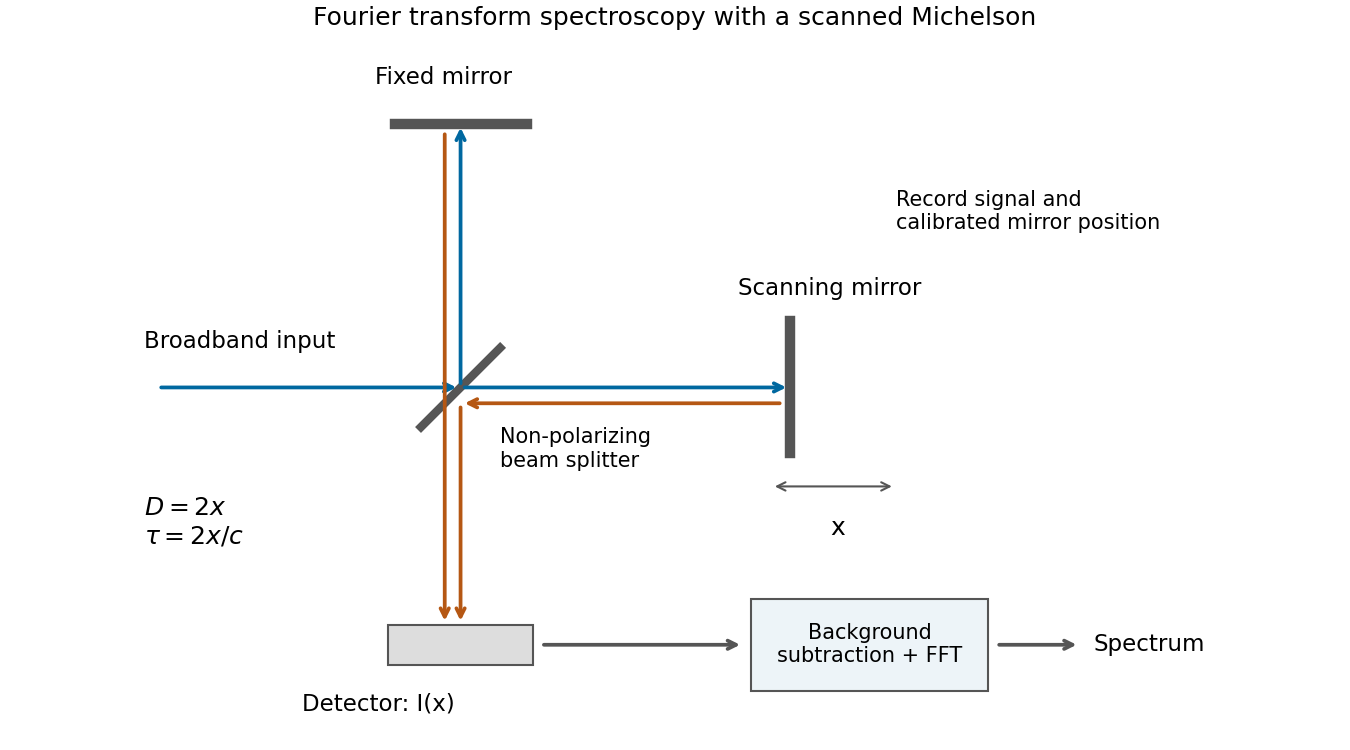
Scanning Michelson spectrometer: mirror position sets delay, and a Fourier transform of the recorded interferogram recovers the spectrum
. Details. 
For matched arm polarizations and balanced throughput, write the ideal signal aswhere is the incident spectral power density and is a constant set by the beam splitter and detector. This is the cosine-transform form of Fourier transform spectroscopy, or equivalently the Wiener-Khinchin theorem applied to delayed self-interference.
The delay-range resolution in Fourier transform spectroscopy follows because recording a finite delay range multiplies the correlation by a window. Its transform broadens each spectral line by an instrumental width of order the reciprocal delay range. A mirror travel range creates a delay range of order , soAt fixed wavelength, absolute wavelength resolution therefore improves inversely with travel range. The numerical coefficient depends on whether is a one-sided or total travel, on the window or apodization, and on whether resolution means first zero, half width or another criterion. The proportionality is the requested convention-independent result. Position sampling must also be fine enough to sample the fastest fringe variation without aliasing.
Let the two arms deliver intensities with unit Jones vectors . For a perfectly coherent input, the recombined intensity under relative phase isConsequently the polarization overlap in interferometric visibility isFor equal returned intensities, two linear polarizations at angle have overlap and thereforeChoose one linear direction as and a circular polarization as . Their overlap has magnitude , givingA non-polarizing beam splitter does not by itself guarantee equal arm losses; if , multiply either boxed polarization factor by . Perfect temporal coherence does not compensate for polarization or intensity imbalance.
For equal line intensities, the correlation is proportional to . The two-line coherence beating envelope is therefore .
In the original first plot, the first visibility zeros are at approximately ; the envelope revives at and about . HenceUse the envelope recurrence or its nulls, not the much faster carrier fringes. The visibility zeros indicate equal component intensities in the ideal model; unequal intensities would leave a nonzero minimum. The arbitrary vertical normalization does not affect the inferred separation.
Interpret the stated as the coherence-decay time, or the mean interval between fully phase-randomizing collisions in the simple impact model of pressure broadening. Then each line has correlation . The collisional phase relaxation and Lorentzian linewidth transform givesThe intrinsic spectrum is the sum of two such Lorentzian line shapes, still centred apart. With equal weights and balanced arms, its normalized visibility isFor the intensity normalization of the first source plot, the corresponding model interferogram isThe constant background remains ; only the oscillatory contrast decays. The beating zeros and recurrence spacing remain fixed, but successive visibility revivals shrink, reaching a factor at and at . Long-delay fringes disappear toward the background.
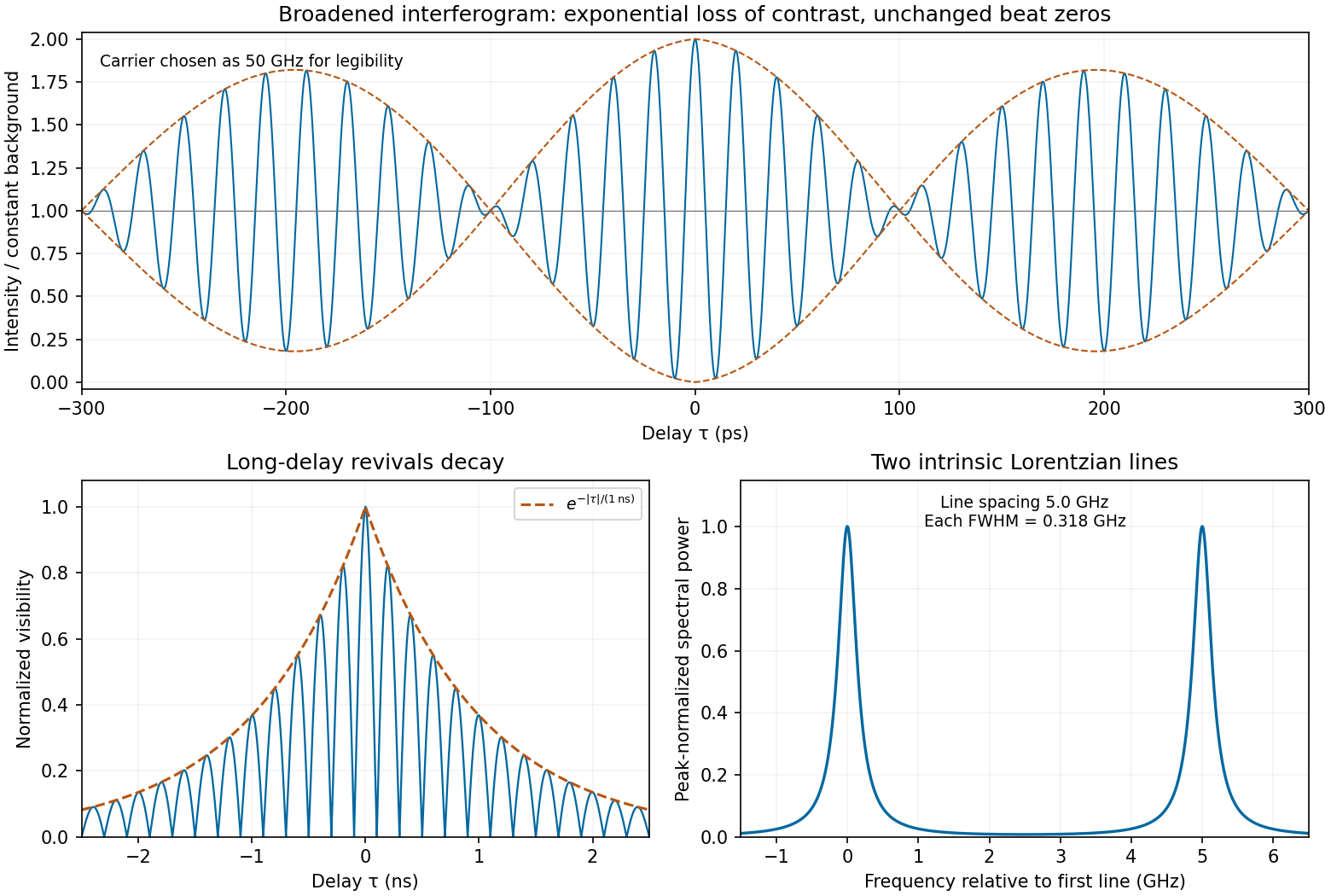
Calculated pressure-broadened interferogram, decaying visibility revivals and Lorentzian doublet for a one-nanosecond coherence time
. Details. 
The sketch chooses a carrier frequency for legibility; the envelope and linewidth follow from the inferred spacing and specified coherence time. A finite experimental delay window additionally convolves these intrinsic Lorentzians with the instrumental line profile. If were instead a population lifetime, the lifetime-limited field decay rate would be and the corresponding linewidth would be half the boxed value. The source does not define that time convention explicitly; pressure-collision coherence decay is the interpretation used here.
For equal-intensity lines of spacing , sum their correlations as a geometric series:The interferogram of an equally spaced spectral multiplet has normalized visibilityIn the second original plot, full revivals occur at approximately , soBetween and there are three zeros, near , and , and two small subsidiary lobes. Since the model has zeros between adjacent revivals,The peak envelope of about and the intensity background of about are consistent with four equal components in the source's normalization, but the internal zero count is the useful shape-based check. The inference assumes the equal spectral weights represented by the graph; revival spacing alone does not fix the number of lines, and arbitrary unequal or hidden components would require more spectral information. Delayed self-interference measures spectral powers, not the relative phases between different source frequencies, so these revivals alone do not prove that the source emits a phase-locked pulse train.
Articles by others on the same topic
There are currently no matching articles.