The supplied PDF is marked as a draft dated 17 May 2018. These solutions follow all five pages of that document.
The London penetration depth measures the density-to-mass ratio of carriers participating in superconducting screening. With electron-counted density and the stipulated bare electron mass ,Using , , and givesThis is the requested conduction-electron density within the assumed local London equation model. More precisely, it is the superconducting carrier density from London screening; identifying it with all conduction Electrons assumes that they participate in screening at the measurement temperature. No temperature-dependent normal-carrier fraction is supplied.
If the condensate is instead counted as Cooper pairs, the pair mass is and charge magnitude is , giving pair density . Keeping Electron and pair counting consistent avoids a spurious factor of two.
At normal incidence, continuity of tangential wave phase makes both internal wavevectors normal to the parallel faces. For the ordinary wave in a uniaxial optical medium, the electric field is an eigenpolarization of the permittivity tensor, so . ThusIts energy path is also normal to the faces. The extraordinary wave differs because but need not be perpendicular to . In a nonmagnetic crystal, and is perpendicular to . The vectors lie in the same meridional plane, with and . Therefore the electric-displacement angle from birefringent walk-off equals the angular separation between and .
The observed lateral separation is accumulated over thickness , so . With and ,The two emergent rays are parallel because their outgoing wavevectors are both normal to the faces in air; their internal energy paths can nevertheless be displaced by birefringent walk-off. The angle quoted is the positive angle between the field vectors, so the unspecified lateral direction does not affect its value. The unpolarized light excites both eigenpolarizations; it does not require their energy paths to coincide.
First obtain the particle speed from kinetic energy rather than treating as its total energy. With Electron rest energy ,For Cherenkov radiation, the photon propagation direction makes angle to the particle trajectory, with . The speed correction is negligible at three significant digits, but the Cherenkov photon-cone and wavefront-cone angles must be distinguished.
If the given opening is the full cone of photon directions, . The result isIf instead denotes the full opening of the conical wavefront, its half-angle is complementary to the photon direction: . That convention givesThe original PDF supplies no cone diagram or definition distinguishing these geometries. Thus the literal full photon-cone interpretation gives , while follows from the wavefront interpretation. It would be incorrect to interchange sine and cosine without stating which cone is meant.
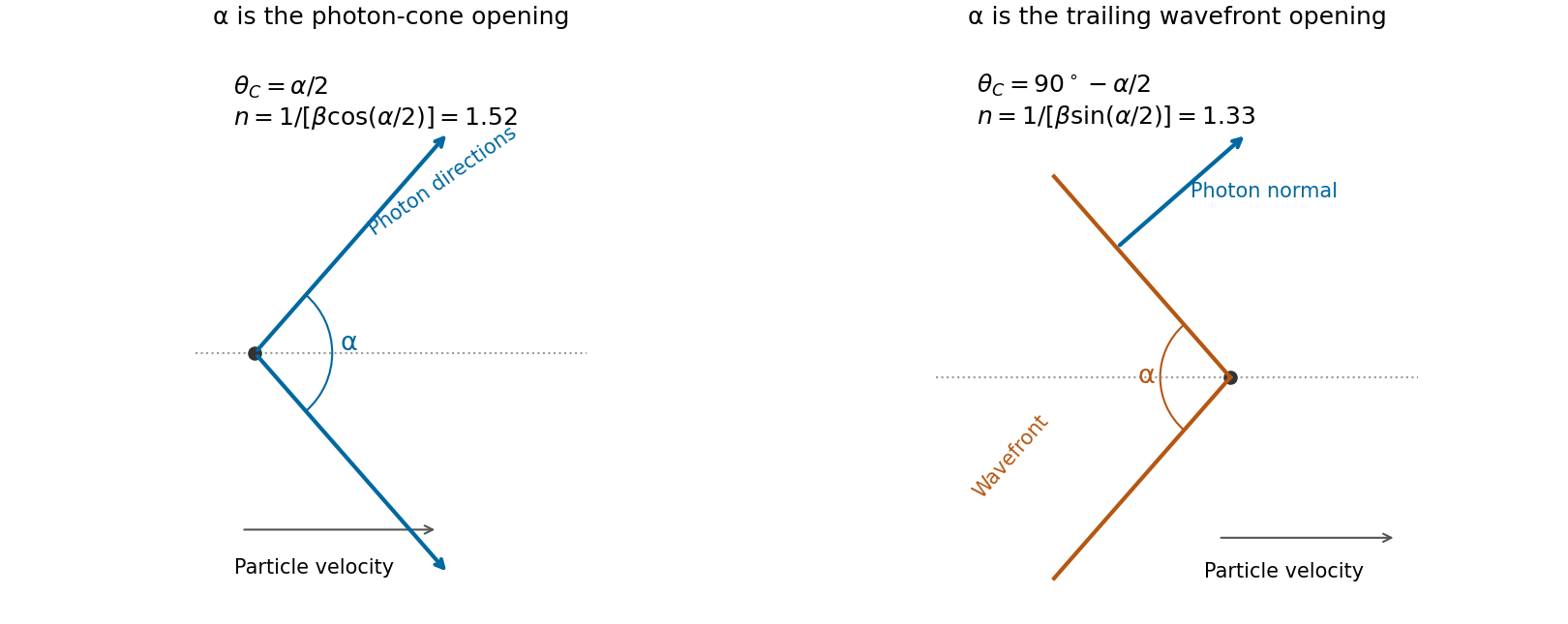
Photon-direction and wavefront cone openings are complementary geometries, giving different interpretations of the supplied angle
. Details. The five tasks below concern a scanned Michelson interferometer. The original dashed curves are labelled visibility in arbitrary units; divide them by their maximum to obtain normalized interferometric visibility, which lies between zero and one.
A non-polarizing beam splitter divides the incident spectrum into a fixed arm and an arm with a translating mirror. Recombining their returned fields gives a detector signal as a function of mirror position . The round-trip optical path difference is relative to the equal-arm position, so the delay is in air approximated as vacuum. Record both detector signal and calibrated position, subtract the constant background, and take a Fourier transform of the interferogram.
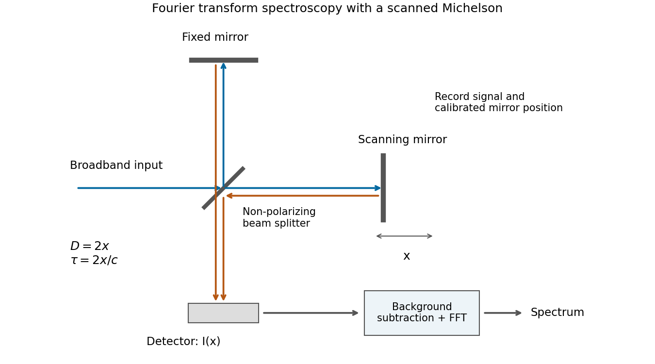
Scanning Michelson spectrometer: mirror position sets delay, and a Fourier transform of the recorded interferogram recovers the spectrum
. Details. For matched arm polarizations and balanced throughput, write the ideal signal aswhere is the incident spectral power density and is a constant set by the beam splitter and detector. This is the cosine-transform form of Fourier transform spectroscopy, or equivalently the Wiener-Khinchin theorem applied to delayed self-interference.
The delay-range resolution in Fourier transform spectroscopy follows because recording a finite delay range multiplies the correlation by a window. Its transform broadens each spectral line by an instrumental width of order the reciprocal delay range. A mirror travel range creates a delay range of order , soAt fixed wavelength, absolute wavelength resolution therefore improves inversely with travel range. The numerical coefficient depends on whether is a one-sided or total travel, on the window or apodization, and on whether resolution means first zero, half width or another criterion. The proportionality is the requested convention-independent result. Position sampling must also be fine enough to sample the fastest fringe variation without aliasing.
Let the two arms deliver intensities with unit Jones vectors . For a perfectly coherent input, the recombined intensity under relative phase isConsequently the polarization overlap in interferometric visibility isFor equal returned intensities, two linear polarizations at angle have overlap and thereforeChoose one linear direction as and a circular polarization as . Their overlap has magnitude , givingA non-polarizing beam splitter does not by itself guarantee equal arm losses; if , multiply either boxed polarization factor by . Perfect temporal coherence does not compensate for polarization or intensity imbalance.
For equal line intensities, the correlation is proportional to . The two-line coherence beating envelope is therefore .
In the original first plot, the first visibility zeros are at approximately ; the envelope revives at and about . HenceUse the envelope recurrence or its nulls, not the much faster carrier fringes. The visibility zeros indicate equal component intensities in the ideal model; unequal intensities would leave a nonzero minimum. The arbitrary vertical normalization does not affect the inferred separation.
Interpret the stated as the coherence-decay time, or the mean interval between fully phase-randomizing collisions in the simple impact model of pressure broadening. Then each line has correlation . The collisional phase relaxation and Lorentzian linewidth transform givesThe intrinsic spectrum is the sum of two such Lorentzian line shapes, still centred apart. With equal weights and balanced arms, its normalized visibility isFor the intensity normalization of the first source plot, the corresponding model interferogram isThe constant background remains ; only the oscillatory contrast decays. The beating zeros and recurrence spacing remain fixed, but successive visibility revivals shrink, reaching a factor at and at . Long-delay fringes disappear toward the background.
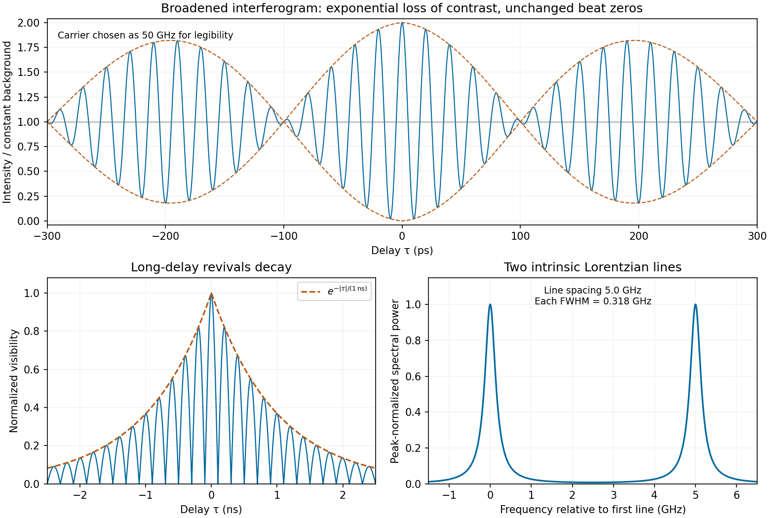
Calculated pressure-broadened interferogram, decaying visibility revivals and Lorentzian doublet for a one-nanosecond coherence time
. Details. The sketch chooses a carrier frequency for legibility; the envelope and linewidth follow from the inferred spacing and specified coherence time. A finite experimental delay window additionally convolves these intrinsic Lorentzians with the instrumental line profile. If were instead a population lifetime, the lifetime-limited field decay rate would be and the corresponding linewidth would be half the boxed value. The source does not define that time convention explicitly; pressure-collision coherence decay is the interpretation used here.
For equal-intensity lines of spacing , sum their correlations as a geometric series:The interferogram of an equally spaced spectral multiplet has normalized visibilityIn the second original plot, full revivals occur at approximately , soBetween and there are three zeros, near , and , and two small subsidiary lobes. Since the model has zeros between adjacent revivals,The peak envelope of about and the intensity background of about are consistent with four equal components in the source's normalization, but the internal zero count is the useful shape-based check. The inference assumes the equal spectral weights represented by the graph; revival spacing alone does not fix the number of lines, and arbitrary unequal or hidden components would require more spectral information. Delayed self-interference measures spectral powers, not the relative phases between different source frequencies, so these revivals alone do not prove that the source emits a phase-locked pulse train.
Use the ideal electrically short Hertzian dipole, , with negligible ohmic loss. Far-field statements additionally require an observation distance large compared with the wavelength and source dimensions. These assumptions distinguish its radiation from near-field coupling and from scattering by a general extended antenna structure.
Choose along . If the end charges are separated by fixed distance , then . The conventional current into the positive end is , soThe current is in phase quadrature with the dipole moment. A different time origin or current orientation changes the sine's sign or phase but not its amplitude. Units check: .
For a dipole along , axial symmetry removes dependence on azimuth . In the Lorenz gauge, its magnetic vector potential points along , so it has spherical components , and . The scalar potential is also independent of . Thus , while taking leaves only an azimuthal magnetic field:The generally nonzero components are . This statement includes the full dipole near field. In the leading radiation zone term, also vanishes; its nonzero full-field contributions fall faster than . Confusing those two levels of approximation would incorrectly suggest four exact zeros everywhere.
For a localized current density, the retarded magnetic vector potential isAt large , replace the amplitude denominator by . For an electrically short dipole, the delay difference across its length is negligible compared with an oscillation period, so evaluate all currents at . The continuity equation for electric charge gives the identitywhere localization makes the boundary term vanish. HenceIn this gauge its Cartesian direction is fixed and its magnitude depends only on and the retarded dipole motion, with spreading. Spherical components have the geometric factors and above; the angular radiation pattern arises after differentiating the potentials, not from an isotropic radiated intensity.
The outgoing radiation field has magnitude and . The radial Poynting vector, averaged over one cycle, givesThus the cut has a two-lobed shape, with zeros along and maxima along . In the plane, throughout and the cut is a circle: there is no azimuthal dependence. At fixed direction the flux falls as , while power per solid angle is independent of observation radius.
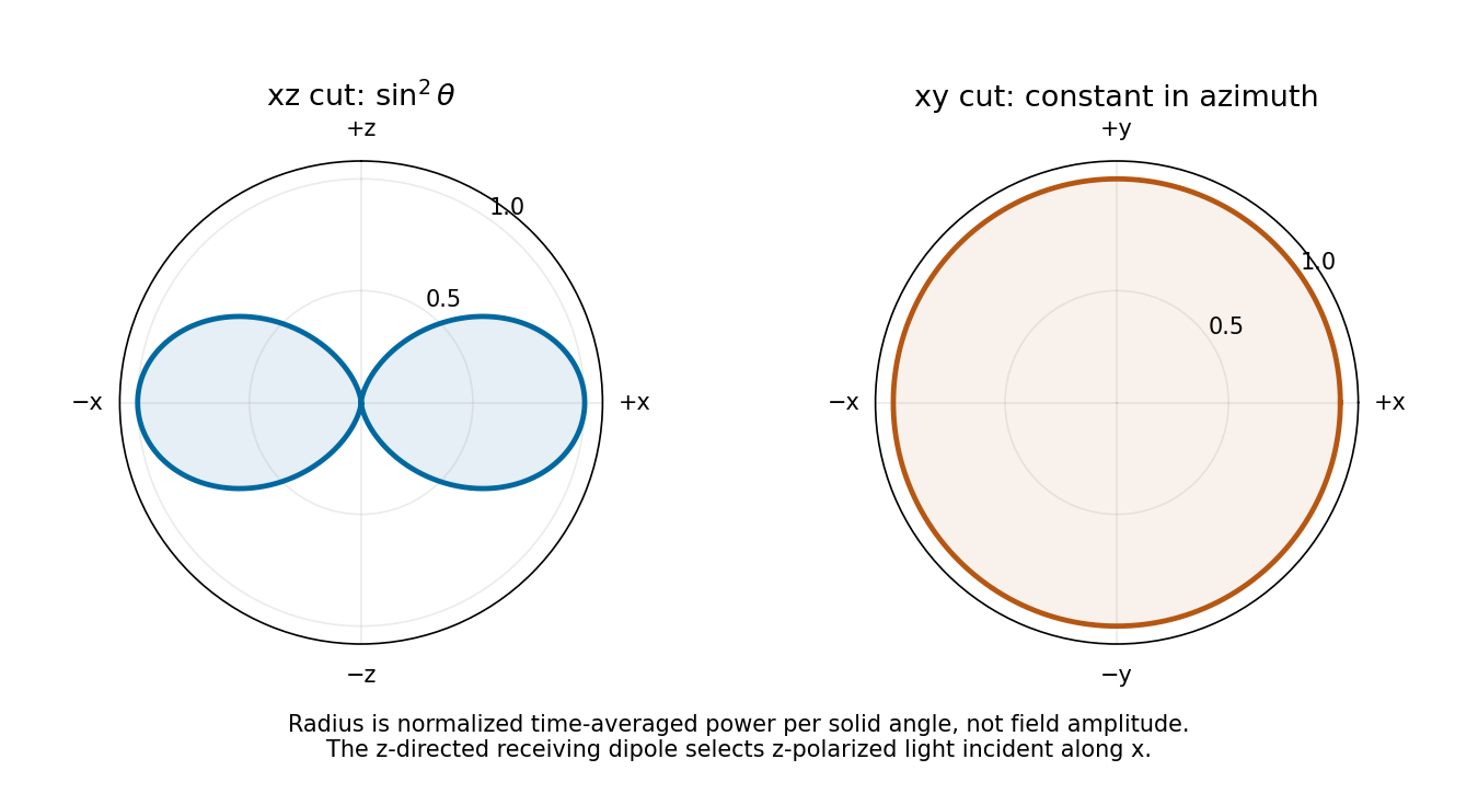


As a receiver for propagation along , the antenna responds to the incident electric field component along . For linear polarization at angle to , the available load power is proportional to : it is maximal for polarization and zero for polarization. Equal incident intensity in circular polarization gives half the matched-linear power. This polarization response follows from the induced voltage's projection along the dipole axis.
Antenna gain in direction compares the far-field power per solid angle with an isotropic radiator using the same accepted input power:It includes radiation efficiency; for the lossless dipole . The antenna effective area is defined for incidence from a specified direction with matched polarization and conjugate impedance matching:Its units are square metres and it need not equal the physical metal area.
For ordinary reciprocal antennas, electromagnetic reciprocity makes the coupling between two matched ports the same when transmitter and receiver are exchanged. Free-space transfer in one direction is proportional to , while the reverse transfer is proportional to . Thus must be a universal factor at that wavelength, independent of antenna or direction. The supplied relation fixes it asEquivalently, thermal detailed balance prevents an angular receiving pattern from collecting more radiation than its reciprocal emitting pattern would return in equilibrium. Reciprocity and the specified matching are the assumptions behind this statement; it is not a general theorem for active nonreciprocal devices.
Integrating the radiation pattern uses , so its lossless gain isThe receiver lies on the axis, broadside to both -directed dipoles. Thus and their linear polarizations match. At , , givingAt separation , the incident flux is . The Friis transmission equation therefore gives the matched-load powerThe far-field and weak-coupling approximations are well satisfied at a distance of about wavelengths for an electrically short dipole. Matching refers to the available received power, not interception of all power in a geometric area equal to the wire's physical size.
The receiving dipole remains matched. To model its actual reradiation, let its feed impedance be with no ohmic loss, and its matched load be . The induced current dissipates equal powers in the load and in radiation resistance. Thus matched-load scattering of a Hertzian dipole has , even though its port is matched.
The scattered wave has the same dipole gain toward the original antenna. Applying the reciprocal link factor a second time gives the reciprocal Hertzian-dipole echo:Each leg supplies an inverse-square spreading factor. This is the carrier-averaged power during a returned pulse with the stated transmitted power during its pulse. The pulse-train average additionally depends on duty cycle, which is not given. Treating the pulses as narrowband keeps the same gain and wavelength approximation.
A matched feed does not make a physical dipole a perfect absorber with zero external scattering. A model retaining only an antenna load-mismatch echo would set its reflected travelling-port wave to zero and would not determine this reradiation. Conversely, an arbitrary antenna structure can add scattering not fixed by gain and effective area alone. The numerical answer uses the ideal lossless Hertzian-dipole scattering model just stated.
Use a boost along the wire axis when comparing frames. The current variable in a four-current must be current density, in , rather than a scalar total current in amperes. For the wire-force calculation it is convenient to integrate charge and current over each cross-section and work with line quantities.
A Lorentz four-vector is a set of four components transforming as under a Lorentz transformation. Examples include the four-position and four-velocity. A Lorentz invariant is a quantity unchanged by that transformation. With metric signature , the scalar product is invariant. The components of a four-vector are generally not individually invariant.
The proton's total electric charge is taken to be a scalar: it does not acquire a factor when the proton moves. Experimental evidence comes from sensitive charge neutrality tests of matter. Hydrogen molecules and helium atoms remain neutral despite different binding and internal Electron and nuclear motions. If constituent charge scaled with kinetic energy as relativistic mass does, the same cancellation of fixed numbers of proton and Electron charges would generally fail in different bound systems.
In a gas-efflux test of charge neutrality, gas escapes from an electrically isolated vessel connected to an electrometer. Any net charge per escaping molecule would leave a measurable opposite vessel charge, after residual ions and charged contaminants are removed. The hydrogen/helium efflux experiment supports velocity-independent additive charge. [ref]
https://doi.org/10.1103/PhysRevLett.5.562. Search for a Small Charge Carried by Molecules (1960), hydrogen and helium efflux measurements
This is evidence for charge invariance, not merely conservation of electric charge: the latter concerns constancy during a process, while invariance compares descriptions or internal motions without rescaling charge by a boost factor. Net-matter neutrality constrains combinations of constituent charges; it should not be described as an exact proof covering every possible velocity-dependent microscopic model.
Let an object be at rest in , with proper charge density and no rest-frame current. In a frame moving at relative to it, the object moves with velocity . A simultaneous volume element is Lorentz-contracted along the motion, , while its charge is invariant. ThereforeThe object's four-velocity in this frame is , soA scalar proper density times a Lorentz four-vector transforms as a Lorentz four-vector, demonstrating the claim. With the alternative convention that denotes the object's velocity in the observer frame, the spatial component is instead. Summing the four-currents of different carrier species preserves this transformation law even when the combined current has no rest frame, as for a lab-neutral current-carrying wire.
A long straight wire carrying current produces field magnitude at a parallel wire a distance away. The magnetic force on a current-carrying wire is . Hence for equal currents,The two forces have equal magnitude and opposite directions. Net electrical neutrality removes a lab-frame external electrostatic force between ideal uniform wires, but does not remove their magnetic interaction.
Put wire 1 on the axis and wire 2 at , with positive pointing away from wire 1. Let each wire have stationary positive linear charge density and moving Electron line density in the lab. For equal currents, both Electron populations have drift velocity , so the signed conventional current is .
First consider wire 2's positive charges in their own rest frame, which is the lab. Wire 1 has zero total line charge there, so its external electrostatic field is zero. The positive-charge force per length is therefore .
Next use the Electron rest frame moving at . Wire 1's ion line density becomes . Its Electron density becomes : the Electron rest density is lower than its lab density. The transformed total isEquivalently this follows from the four-current transformation , with and . By the electrostatic field of a line charge,A wire-2 Electron is at rest in and feels only the electric force, , toward wire 1.
Apply the supplied transverse relativistic force transformation with the Electron's lab velocity . Its denominator is , so , or . There are Electrons per unit lab length. ThusAdding gives exactly the attractive magnetic result. This electrostatic-frame derivation of parallel-wire forces uses electrostatics in each test carrier's own rest frame; no magnetic force acts on that stationary test carrier there. The other wire can still carry current in that frame. Transform the force per Electron first and then count Electrons per lab length: transforming a force per unit length as if it were a particle force would introduce an incorrect extra contraction factor.
Keep wire 1's Electrons moving at , but let wire 2's Electrons move at , so . The positive charges remain lab-stationary and still feel zero external electrostatic force in the lab. The appropriate rest frame for wire 2's Electrons now moves at .
In this frame, wire 1's total line charge isIt produces an electric field pointing toward wire 1. The stationary test Electron is negatively charged, so its electric force points away from wire 1. Transforming back again divides the individual transverse force by , and multiplying by givesThe changed sign arises from the changed transformed charge imbalance, without needing a magnetic-force calculation. More generally the signed result is for the chosen outward radial direction.
Articles by others on the same topic
There are currently no matching articles.