The emission mechanism is Cherenkov radiation. An Electron moving faster than the phase velocity of light in the material excites electric polarization disturbances whose radiation adds coherently on a cone. This does not require the Electron to exceed the speed of light in vacuum. Taking as constant over the detected optical band, the Cherenkov cone angle satisfiesEmission requires . The detector accepts , soNumerically,The lower endpoint has vanishing Cherenkov radiation yield, and the upper endpoint is excluded by the stated strict angular acceptance. Faster Electrons emit at larger cone angles: at , , outside this detector's acceptance. The angular condition gives the accepted speed interval conditional on rays reaching the detector; no collection geometry or total signal yield is specified.
The Johnson-Nyquist noise formula gives the open-circuit mean-square voltage in a small frequency band . When a source electrical resistance drives a load with impedance matching, the load sees half the source voltage, so the available noise power isThe factor of four in the open-circuit formula is therefore not an extra factor in the delivered power.
The transmitter's antenna gain makes the axial spectral energy flux at range Multiplication by the receiving antenna effective area gives . Define the equivalent receiving antenna temperature by the available matched-load noise . ThenThis is the transmitter-induced equivalent noise temperature of the receiver port. It does not determine the actual physical temperature of its internal electrical resistance, or any additional receiver and background noise. The calculation assumes the usual far-field link, negligible path loss beyond geometric spreading, matched polarization of an electromagnetic wave at the two antennas and the stated effective collecting area. No additional one-half polarization factor is needed for the matched polarization of radiation from one transmitting antenna.
Each mutually incoherent patch of an extended star produces a displaced double-slit interference pattern. The detector adds their light intensities. For two apertures separated by a projected interferometric baseline , a source direction offset by a small angle changes their phase difference by . The normalized sum over the source's angular brightness distribution is its first-order optical coherence, whose magnitude is the interferometric visibility for equally bright channels.
For a uniform circular stellar disk of full angular diameter , the normalized angular Fourier transform gives the uniform-disk stellar visibilityHere is the order-one Bessel function of the first kind. This follows by integrating over the disk and dividing by its area. In particular, its power series gives .
For an ordinary slit separation , using the paper's and observing wavelength ,Even gives a visibility loss of only . Thus millimetre separation leaves the interference fringes almost indistinguishable from those of a point source; it gives very little sensitivity to the diameter.
The movable mirrors in the Michelson stellar interferometer collect light at a large adjustable separation and redirect it into closely spaced output beams. They increase the sampling interferometric baseline independently of the fixed output slit spacing : sets sensitivity to source structure, whereas the output optics set the screen's interference fringe spacing. The first Bessel function zero is , henceThe interference fringes disappear at this baseline even though each beam separately remains bright.
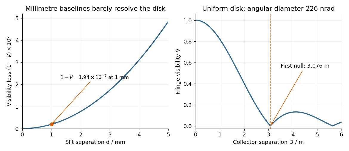
The value assumes a uniform disk. The original question supplies a diameter without a surface brightness law; real limb darkening changes the precise visibility zero. A one-dimensional uniformly bright strip of the same full angular width instead has a sinc function visibility and first zero . That is a different source model, not the circular-disk result. The robust conclusion without a surface brightness model is that a baseline of a few metres, rather than millimetres, is required.
Birefringence means that two independent polarization eigenmodes have different refractive indices at the same frequency and propagation direction. The rotatory-power formula relevant here requires circular birefringence: the eigenmodes are opposite circular polarizations. General linear birefringence instead introduces phase retardation between linearly polarized components and need not rotate every incident linear polarization through one common angle.
Use the complex amplitude convention and transverse unit vectors . DefinePropagation through thickness adds phases , where is the vacuum wavelength. Recombining the two components givesThus the rotation and the specific rotatory power per unit length areThe units of are . The sign follows the specified circular basis and viewing convention. Equal attenuation of the two eigenmodes has been assumed; unequal attenuation also produces elliptical polarization.
Flint glass is approximately optically isotropic without an applied magnetic field. A longitudinal magnetic field changes the motion of its bound Electrons: the magnetic part of the Lorentz force acts with opposite sense on the two circularly rotating components of a driven electronic oscillation. Their optical response, and hence their refractive indices, split. Equivalently, the transverse permittivity tensor acquires a field-odd antisymmetric contribution whose eigenvectors are opposite circular polarizations.
The resulting circular birefringence gives Faraday rotation. For a weak longitudinal bias it is linear in the field:Here is the Verdet constant and the path length. The magnetic field breaks time-reversal symmetry, which is why this rotation is nonreciprocal. Reversing the bias reverses the rotation; reversing propagation while keeping the bias fixed does not undo it when physical polarization directions are compared in fixed laboratory axes. A transverse magnetic bias can have different, higher-order effects; the setup here is the longitudinal Faraday effect.
Choose the first polarizer's pass axis as and write the second as . The positive signed rotation takes toward by the short angle. Let be signed according to . The Jones matrices of ideal polarizers are their orthogonal projection matrices,Removing the unimportant common propagation phase, the lossless glass block has the rotation matrixThe elements act from right to left, soWith the common optical phase retained, multiply this by . Extra scalar attenuation would also multiply the result, but none is supplied. A single Jones vector does not represent unpolarized light; the device's Jones matrix is nevertheless well defined for each incident component and can be applied to their statistical mixture.
Let be the incident light intensity. The first ideal polarizer transmits and produces linear polarization along . Faraday rotation turns that direction through , and Malus's law at the second polarizer givesEquivalently, use the input coherency matrix and . This produces the same one-half factor required by unpolarized light.
Maxima satisfy , with . For and , the smallest field magnitude isIts direction is the axial direction that rotates the polarization passed by toward the pass axis of through the shorter . In the right-handed ray-basis convention where and the depicted second axis is , this is , along . Reversing that field at the same magnitude gives and zero transmission. A signed Verdet constant is meaningful only together with its rotation convention, so the polarization-alignment description fixes the physical direction without relying on ambiguous clockwise labels in a perspective diagram.
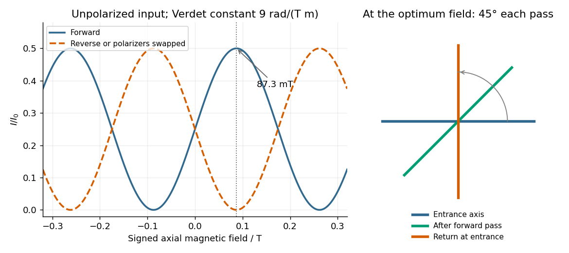
Original forward and reverse transmission curves and laboratory polarization directions at the optimum Faraday rotation
. Details. Keep the magnetic field fixed in the laboratory and exchange source and observer. The incident unpolarized light now meets first. In fixed transverse laboratory axes the backward glass map is still , not : this is optical nonreciprocity of the Faraday effect. The order of the two polarizers is reversed, soThe reverse light intensity is thereforeFor the optimal forward setting , it vanishes: the input selected by rotates to and is blocked by . At a general field, . The result assumes equal incident light intensities in the two experiments. Treating the glass as a reciprocal natural optical rotator would predict cancellation of its laboratory rotation on reversal and would give the wrong answer here.
Keep source, observer and magnetic field in their original places, but interchange the physical polarizers, including their pass-axis orientations. The forward order is then , glass, , so the new Jones matrix is again . ConsequentlyThis is the same intensity change as exchanging source and observer. At the field that maximizes the original forward transmission, the swapped arrangement blocks the beam. If both operations were performed together, the original order relative to propagation would be restored and so would the original transmission. The answer concerns exchanging the two differently oriented pass axes; simply relabelling two identical polarizers while leaving their axes fixed would not change the apparatus.
Only the fields transport a nonzero outgoing power to infinity. Retain those terms from the Hertzian dipole fields:The brackets mean evaluation at the retarded time,for a point source at the origin in vacuum. They are not a time average. The radial Poynting vector in the radiation zone isIntegrating over a sphere usesThereforeNear-field terms either give inverse powers of after the surface integral or describe reversible exchange with the near field. The emitted power labelled by source time is ; the enclosing surface receives it one light-travel time later. For a changing dipole orientation, the general form is .
The prescribed surface charge density is that of a uniformly polarized sphere and has zero total charge because . Its electric dipole moment at isThe transverse components cancel by axisymmetry, while the component isThusThe angular surface distribution is a pure degree-one spherical harmonic. Hence its static external electric potential is exactly that of this dipole, with no higher electric multipole moments; it is not an assertion that the potential inside the finite sphere equals a singular point-dipole potential.
For right-handed uniform rotation about , the rigidly attached dipole isConsequently is constant. The electric dipole radiation formula givesThere is no extra factor of one-half: the squared sine and cosine contributions of the two perpendicular oscillating components sum to one. This is the leading electric-dipole approximation for radiation, requiring and observation in the radiation zone. The stated permanent surface distribution is interpreted as the actual charge producing the given external dipole; adding another dielectric screening factor would contradict the dipole moment the question asks to establish. The relative permittivity enters the induced-polarization problem in part (d), not this prescribed total dipole moment.
Let be the sphere's mechanical moment of inertia about its rotation axis, and let . For an undriven rigid sphere the rotational energy is . In the weak-radiation-loss approximation, conservation of energy givesIntegrating givesEquivalently, the characteristic spin-down time isThe radiative spin-down of a rotating electric dipole therefore has angular frequency that decays as at late times within this model, rather than exponentially. The original paper gives no mass or mass-density profile, so cannot be determined from and the relative permittivity. If a homogeneous solid sphere of mass is additionally assumed, insert ; uniform dielectric response alone does not imply this mechanical mass distribution.
The approximation is important. If the dipole angle is with , direct differentiation gives . Using the constant-frequency radiation law instantaneously neglects the second term and assumes . This gives the standard leading slow spin-down solution above. An exact nonadiabatic radiation reaction evolution would require the mechanical and near-field dynamics beyond the information supplied, rather than treating this leading law as exact at arbitrarily rapid damping.
The given static induced surface charge and the dipole integral from part (b) giveHere is the dimensionless relative permittivity, as required by the stated expression; is the SI electric polarizability. Take and . In the Rayleigh scattering regime the field is approximately uniform across the sphere. Its induced dipole radiates mean powerThe incident time-averaged light intensity in vacuum is . Dividing power by intensity gives the total cross section,The units are ; the comparison is with the geometric projected area , not with a length:The inequality holds for an ordinary nonabsorbing dielectric, with finite contrast factor and . It explains why a sufficiently small transparent sphere scatters weakly and why its scattered power has the characteristic dependence. Near a material resonance where is small, this simple inequality and static-polarizability approximation need reconsideration, including loss and radiative corrections. For the stated low-frequency ordinary dielectric the supplied polarizability is the intended approximation.
Fix coordinates and use the following convention for the contravariant electromagnetic field tensor:For moving with velocity relative to , the Lorentz transformation hasThe rank-two tensor transformation rule isFor example,Similarly, and . The component is unchanged because , and the component is unchanged since neither index lies in the boost plane. Reading off the six field components givesAn alternative overall sign convention for gives the same physical Lorentz transformation of electromagnetic fields when its identifications with and are used consistently.
Write , , and , evaluated at the same transverse coordinates . A superscript labels each filament's own rest frame, rather than a single common frame in all cases. The filaments are infinite and uniform along , so the change of longitudinal coordinate under a Lorentz boost creates no extra dependence in these functions. After the acceleration transients have passed, the magnetic field of each filament vanishes in its own rest frame.
For a filament moving at , use the inverse of part (a): its transverse electric field in the laboratory is and its magnetic field is . Superposition for the two co-moving filaments therefore gives, in ,In the common co-moving frame both filaments are at rest, soFor example, , a useful sign check. The supplied is the proper linear charge density. Thus each laboratory density is and each laboratory electric current is , consistently with length contraction and the four-current transformation. In each density is and both currents vanish.
Retain as defined in Case 1. In the laboratory, A moves and B is stationary. Transform A's fields and add B's unchanged electrostatic field:The laboratory linear charge densities are and , with electric currents and .
In , A is stationary while B moves with velocity . Thus A contributes its rest electrostatic field, and B contributes the boosted electric field and the opposite-sign convective magnetic field:The densities in this frame are , , with and . Substituting the laboratory result into part (a) gives the same fields; for instance . The magnetic contribution attributed to A disappears in its own frame, but B's contribution does not.
The infinitely long filaments have no finite total force; the meaningful result is force per unit length in the laboratory. Evaluate only A's field at B, excluding B's singular self-field. B is at , so defineIn both cases A moves at , hence at BFor a filament with linear charge density and convective electric current , the Lorentz force per laboratory length isIn Case 1, and . Electric repulsion and magnetic attraction givesoThe cancellation uses . In Case 2, B is stationary, and , givingBoth results have units and are repulsive, away from A, irrespective of the common sign of . In Case 1 the velocity independence of force per laboratory length does not violate the transverse force transformation: a material segment of proper length occupies laboratory length , so its force is the rest-frame force divided by . The calculation interprets the stated as each filament's final proper density; holding a laboratory density fixed during acceleration would be a different preparation.
Spin-orbit coupling is a relativistic interaction between a particle's spin and its orbital angular momentum or, more generally, its motion through an electric field. A moving Electron experiences a transformed magnetic field, which couples to its magnetic dipole moment. For an electron bound in a central electrostatic potential energy , the leading interaction, including the Thomas precession correction, isHere is orbital angular momentum and is spin. The factor of one-half relative to the simplest rest-field argument comes from Thomas precession of the accelerated Electron frame.[ref]
Topics in Quantum Mechanics by David Tong. §3.1.3, printed pp. 71–75: rest-frame magnetic interaction and Thomas correction
For example, in the hydrogen atom, the states with total angular momentum and have different eigenvalues. Their splitting is part of the atomic fine structure. The interaction redistributes and splits spin-dependent energies; it is not the same physical effect as the spin-independent convective magnetic force between charged filaments.
The information in the original question is insufficient to determine a unique spin-induced change of charge density. It specifies ideal dielectric filaments with a prescribed excess linear charge density, but not the charge carrier species, their spin state, charge carrier mobility, binding potential or relaxation mechanism. A classical line charge has no spin variable at all. The following conditional conclusions are supported by the fields already calculated.
For a carrier moving with its filament, the local magnetic field in its instantaneous rest frame is, for the transverse fields here,where is that carrier's laboratory velocity. Exclude its filament's singular self-field and first retain only the prescribed straight convective motion.
In Case 1 there is a common rest frame in which both filaments and the excess charges are stationary and the interfilament magnetic field vanishes. Equivalently, in the laboratory , so B's co-moving charges have . Thus uniform common translation alone creates no extra mutual rest-field spin splitting. This does not exclude intrinsic spin-orbit coupling of electrons moving within their atomic binding potentials; that material physics was never specified.
In Case 2 there is relative motion and no frame in which both source distributions are stationary. Put as in part (c). At the respective filament axes, the external fields experienced in each carrier distribution's own rest frame areFor the first expression B is at rest in ; for the second A is at rest in and the field comes from B moving at . For a carrier with magnetic dipole moment , the interaction distinguishes opposite transverse spin orientations. A field gradient could exert a spin-dependent force on mobile carriers; spin relaxation could instead produce a spin polarization. These are possible responses, not consequences of charge density alone. In B's frame the displayed interaction is directly a magnetic-moment coupling to the moving source's field; treating the moving carrier's electrostatic orbital term in another frame also requires consistent binding and acceleration dynamics, including any applicable Thomas precession.
For example, if and mobile electron spins can relax, the lower magnetic-energy orientation has the electron's magnetic moment toward and its spin toward . Oppositely oriented moments would experience opposite gradient forces. The sign changes if the source charge changes sign. None of these statements fixes a net charge redistribution without a confinement and response model, and the stipulated zero transverse size supplies no resolved “sides” on which charge could accumulate.
Therefore Case 1 has no new mutual spin effect from common bulk motion alone; Case 2 permits motion-induced spin-dependent interactions, but neither case determines an additional charge-density profile from the supplied data. In particular, the factor relating proper and laboratory linear charge densities in part (b) follows from length contraction and is not an effect of spin-orbit coupling. If the charges remain pinned in an ideal dielectric, their imposed density remains the prescribed density in either case.
Work in the dilute, single-scattering limit and add the diffuse scattered light intensities of randomly positioned particles. The incident unpolarized light has equal, mutually uncorrelated and electric components. Each particle therefore has an induced electric dipole moment along its permitted axis, with the same mean squared magnitude proportional to .
For an observer in direction , choose transverse unit directions in the scattering plane and perpendicular to it. The electric dipole radiation field is proportional to the transverse projection of the electric dipole. Hence an electric dipole contributes a wave amplitude factor along , while a electric dipole contributes its full wave amplitude along .
Let collect the common incident light intensity, electric polarizability, distance and frequency factors. ThenThe two components are uncorrelated, so the coherency matrix is diagonal in this basis. The degree of polarization isA signed degree of linear polarization, defined positive perpendicular to the scattering plane, has the same expression without the absolute value. The dominant direction is when , and when the inequality reverses. If the denominator vanishes there is no scattered signal and its degree of polarization is undefined. A coherent exactly forward component, including the transmitted incident beam, is not part of this diffuse-intensity calculation; random particle positions do not by themselves destroy forward optical coherence.
Now take , with the same angle to the incident direction. The perpendicular direction is and the in-plane transverse direction is . The roles of the two electric dipole populations interchange: electric dipoles radiate at full strength, whereas the observed wave amplitude from a electric dipole is reduced by .
Thus and , givingThis is also obtained by the symmetry , in part (a). For , both planes give the familiar Rayleigh scattering degree of polarization : the diffuse signal is unpolarized forward and fully linearly polarized at right angles. At a dark direction with zero denominator, no degree of polarization can be measured.
The transmitting antenna is matched to its input transmission line, so its real terminal electrical resistance is . The identical receiving antenna has the same electrical impedance at the operating frequency. Its available received power for a matched load is the incident energy flux times its antenna effective area:The real receiving load is , so its voltage-wave reflection coefficient relative to is . The fraction of available power delivered to the output line isConsequently, neglecting path losses, mismatch of polarization of an electromagnetic wave and line losses,This is the Friis transmission equation with a receiving impedance-mismatch factor. For fixed , it scales as . That scaling is conditional on holding antenna gain fixed: a fixed physical aperture can instead have , and any wavelength dependence of the impedances also enters the expression. The matched-output check gives .
Distinguish reflection at the input terminal, reflection at the receiving load, and a returned signal that traverses the free-space link twice. The input antenna is initially matched, so its direct terminal reflection is zero.
In the usual weak-coupling, matched-port two-port network model for the antenna pair, let the forward and reverse wave amplitude transfer coefficients be and . Electromagnetic reciprocity gives equal power transfer factors , where from part (a). The receiving-load reflection returns wave amplitude to the original input port. The load-mismatch contribution to the returned power is thereforeFor fixed gains and impedances this returned power scales as : it contains two link traversals. By contrast, the reflected power at the receiving load before that return traversal is . Calling that local reflected power the power already back in the input line would omit one propagation loss.
The original wording does not specify an antenna scattering model. The boxed result is the load-dependent echo in an ideal matched-port link, with structural scattering and residual input coupling neglected. The actual total input return can include coherent scattering from the receiving antenna even when ; gains and effective areas alone do not specify that background. If “reflected back” means only the direct reflection at the stated matched transmitting antenna, its value is . These meanings should not be conflated; the result requires the two-pass echo interpretation and its stated model.
After field electron emission, let denote the plate separation of the parallel-plate capacitor, which the question does not specify. The uniform capacitor electric field has magnitude , and a nonrelativistic Electron of mass has constant acceleration magnitude . The sign of its charge affects the direction of the radiation field but not its radiated power.
In the supplied nonrelativistic Liénard-Wiechert field, . At polar angle to the acceleration, , henceThe outgoing Poynting vector has magnitude . Its radiated power per solid angle is thereforeUsing gives the Larmor formula and the requested constant power during the uniform-field part of the flight:The brackets in the given field require the acceleration at retarded time; the radiation reaches the far observer after the propagation delay. This derivation assumes that radiation reaction is a small correction to the acceleration and that the flight is nonrelativistic, for example for release from rest. Entry, emission and impact transients are not described by the uniform-field model. A result solely in terms of cannot be obtained without a plate spacing or a specified internal field.
The characteristic polynomial of the given Jones matrix isso a convenient choice of eigenvalue labels isDirect multiplication gives , and . They represent opposite circular polarizations. Since are real, is a Hermitian matrix and both eigenvalues are real, but they need not be positive. A negative eigenvalue adds a wave phase reversal to that mode. The labels are algebraic: is the larger numerical eigenvalue only when . If , the eigenvalue is degenerate and every nonzero Jones vector is an eigenvector; the circular pair remains a valid basis.
Take an incident field along , without loss of generality because this component has the same circular eigenmodes for every direction of input linear polarization. Resolve its Jones vector into equal circular components:Using the complex amplitude convention , the real circular contributions areThey counter-rotate and add toIn general the tip traces an ellipse with semiaxis lengths and . Equal transmitted circular wave amplitudes produce a line; removal of one circular mode, or , produces a circle. The special zero-output case has no defined polarization of waves.
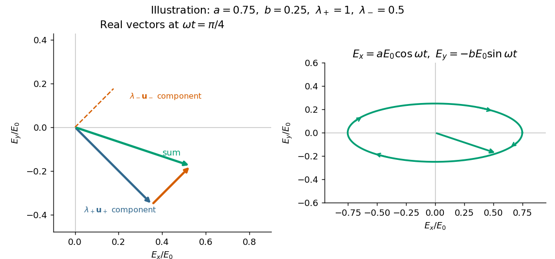
The normalized circular eigenvectors from part (a) define the orthogonal projection matricesThus the spectral decomposition of the Jones matrix isThis simply substitutes and and makes each eigenmode's wave amplitude transmission explicit.
There are errors in the original PDF at this point, not merely in the TeX transcription. The second exponential must denote the eigenvalue , not the propagation coefficient itself. More substantially, the printed prefactor is inconsistent with the stated exponential eigenvalues. It must be . The original's primed Jones-matrix label distinguishes the distributed component from the earlier static matrix; below write to avoid confusing that prime with a derivative.
Complex eigenvalues have no intrinsic largest/smallest ordering, so and are modal labels. Keep the circular eigenvectors fixed, put and , and use the spectral decomposition from part (c):Its diagonal entries are , and its upper off-diagonal entry is . ThereforeWhere , this can be factored asThe unfactored expression is valid even at zeros of the cosine-like factor when is imaginary. The printed expression is times this correct matrix; its eigenvalues are consequently rather than those specified. A second check is , whereas the printed version has determinant . Thus the requested printed identity cannot be proved except in the degenerate case ; the following parts use the consistent propagator.
When are real, and are real. The two opposite circular polarizations retain their wave phases but are attenuated at different wave amplitude rates. This circular dichroism changes the ellipticity without rotating the principal axis of the ellipse.
For input , the corrected Jones matrix givesThe common factor describes the mea wave amplitude attenuation. The factor reflects the sum of the two transmitted modal wave amplitudes; fixes their imbalance and hence the signed ellipticity. The real field has components proportional to and , soThe ellipse's principal axis stays along the original input direction. For large differential optical depth it approaches the less attenuated circular eigenmode. A passive medium has , or , so the growing hyperbolic function factor does not imply net optical gain. Using the printed prefactor would give a spurious extra attenuation inconsistent with the modal laws.
Write , and . Then and . With and , the corrected matrix becomesThe scalar is a common propagation wave phase and the real rotation matrix rotates the input linear polarization through . There is no attenuation and no generated ellipticity: the field map is a unitary matrix. The two circular eigenmodes accumulate different wave phases, giving circular birefringence and optical activity.
The correct unfactored matrix remains finite where . In contrast, the printed form would give times the rotation matrix, including unphysical divergent gain in this stipulated lossless case. This provides a direct physical check on the correction in part (d).
The circular eigenmode orthogonal projection matrices obey , and . Define the uniform-medium generatorExpanding its matrix exponential by its power series and using these projection identities givesEquivalently, with , one has , and . This is exactly the corrected matrix of part (d). The entries of have units of inverse length, and the map satisfies , and the homogeneous propagation law .
The extra factor in the printed version violates this last law for nonzero , so it cannot be generated by one constant with the stipulated eigenvalues. The constant- description assumes uniform coefficients and fixed circular eigenmodes.
Take at a fixed reference point, and define the full-field temporal optical coherence function byThe angle brackets denote an ensemble expected value, or a sufficiently long time average when justified. The factor puts in light intensity units for the chosen peak complex-field convention. The normalized first-order optical coherence is for a stationary source.
“Independent of absolute time” means the second moment depends on the time difference but not on the starting time : shifting both observation times by the same amount leaves it unchanged. Together with a constant mean this is second-order or weak stationarity; it does not mean that the random electric field is constant in time. Put . The full-field convention is important: an envelope-only correlation omits and must have that carrier factor restored before deriving optical interference fringes.
The given spatial and carrier factors combine into retarded copies of the same random field:On the axis, and . Expand the squared electric-field wave amplitude. Each self term contributes , and the two cross terms together contribute the real part of the full-field correlation. Stationarity and giveIn vacuum, and . Reversing the delay convention replaces by without changing this real-part result. This is the electric-field light intensity convention of the question. For two nonparallel waves it should not automatically be identified with the magnitude of the net Poynting vector; part (d) gives that geometric conversion explicitly.
A line with lifetime broadening has a Lorentzian line shape. Write its half-width at half-maximum in angular-frequency units as . The Wiener-Khinchin theorem, or the Fourier transform of the Lorentzian, givesTherefore in vacuumThe sketch is a cosine fringe pattern about baseline , bounded by . Its central value is , its spatial interference fringe spacing is , and its visibility decays on length . For an isolated transition whose population lifetime is and which has no extra dephasing, , so the field coherence time is , not . Introducing avoids confusing population, wave amplitude and spectral-width conventions when no numerical linewidth is given.
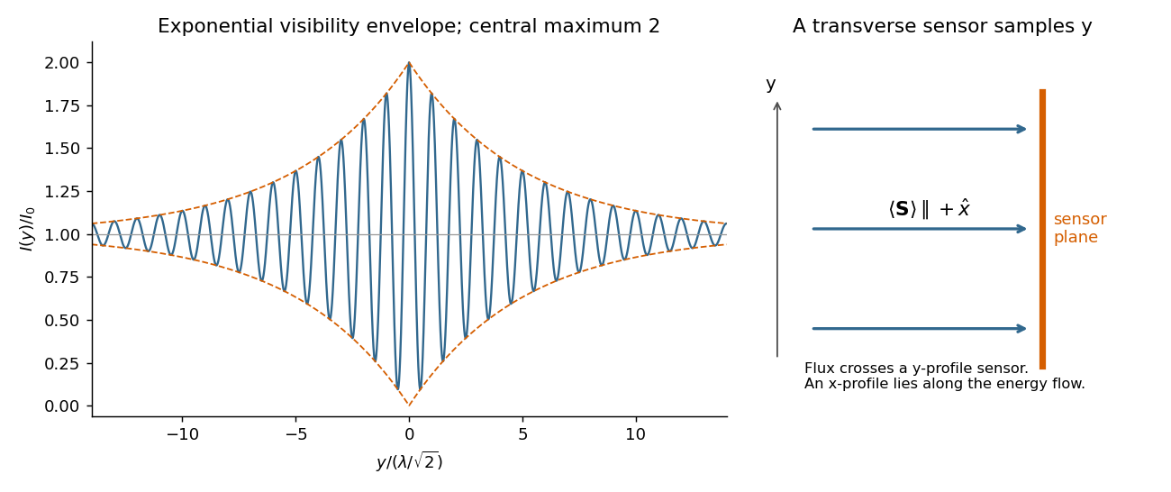


For each beam in vacuum, its magnetic field is . Write the two complex scalar contributions, including the beam splitter factor, as and . Since their electric fields are both along ,The optical-cycle and ensemble-averaged Poynting vector isThe mean individual light intensities are equal, soThus energy flows along the bisector of the two beam directions, crossing a detector plane normal to . Such a sensor can in principle record the variation across its coordinate. Its actual normal energy flux is in the normalization used above; this fixed factor does not change interferometric visibility.
There is a practical resolution condition in addition to the direction of energy flow. The interference fringe spacing is very small, so direct pixels would need spacing no larger than as required by the Nyquist–Shannon sampling theorem, or optical magnification and sufficient angular aperture to preserve both incident directions. An ordinary optical camera with much larger effective pixels averages the interference fringes. The Poynting-vector argument establishes the allowed measurement geometry, not guaranteed resolution with any optical camera.
On the axis the two geometric delays are identical:Their field wave amplitudes therefore add as equal copies at zero relative delay. Stationarity removes dependence on the common delay, givingindependent of in the ideal overlapping plane-wave region. The corresponding mean normal energy flux through a transverse plane is . There is no increasing path difference along the bisector, so finite temporal optical coherence does not produce a longitudinal visibility envelope on this axis.
The axis lies along the mean Poynting vector. A two-dimensional optical camera sensor intended to sample many positions at once would have to lie along the energy flow, where it receives no normal flux in the ideal geometry; a side-view optical camera also sees no light from an empty nonscattering propagation region. Putting a detector normal to measures one transverse section instead, and absorbs the light before a downstream detector can sample the same rays.
One could translate a detector to successive positions or introduce a scattering screen, but that is a different measurement. Moreover the ideal result here is already the constant , so it contains no longitudinal optical coherence structure for the optical camera to resolve. The difficulty is the longitudinal sampling geometry, rather than a hidden -fringe period.
A physical delay is a time, whereas the stated is a length. First interpret it literally as an additional optical path length in arm 1, with the other arm unchanged. In vacuum this delays its full field by . The exact stationarity argument from part (b) then givesDelaying arm 2 changes the plus sign before to a minus sign. As a function of , the arm-1 result is the old pattern evaluated at .
For a quasi-monochromatic source, is much shorter than the coherence time. The envelope correlation can then be treated as unchanged, while the carrier wave phase cannot:HenceThis literal optical-path delay is not a quarter-cycle wave phase shift. If the intended length instead specifies a displacement of the entire recorded fringe pattern by one quarter of its period, , the equivalent delay is and the wave phase shift is . Under that different interpretation the narrow-band result is , with its sign reversed for the opposite displacement. The exact expression is still a shifted argument of , not merely a wave phase multiplier when the envelope varies. The original wording does not specify such a fringe-pattern displacement, so these interpretations must be distinguished.
The upper index identifies as a contravariant Lorentz four-vector, obeying the rank-one contravariant tensor transformation law. Its components transform with the coordinate Jacobian,It is not invariant component by component. Its contracted square , for metric signature , is a Lorentz invariant. This distinguishes a contravariant transformation law from an invariant scalar.
First lower the index of the four-current with the Minkowski metric: . The displayed expression is thenThereforeIts one free lower index transforms with the inverse coordinate Jacobian. The contraction with the metric here lowers an index; it does not make the current a scalar because the index remains free.
The chain rule givesThusDifferentiation with respect to a contravariant coordinate has a lower transformation index. In inertial Cartesian coordinates in Minkowski spacetime, no connection term is needed for this coordinate transformation of a derivative acting on a scalar; Lorentz transformations have constant Jacobians.
Articles were limited to the first 100 out of 192 total.
Articles by others on the same topic
There are currently no matching articles.