Past exam of the short options paper shared by Prelims and Parts A and B of the physics course of the University of Oxford / 2012 / S25 / 3 / 4

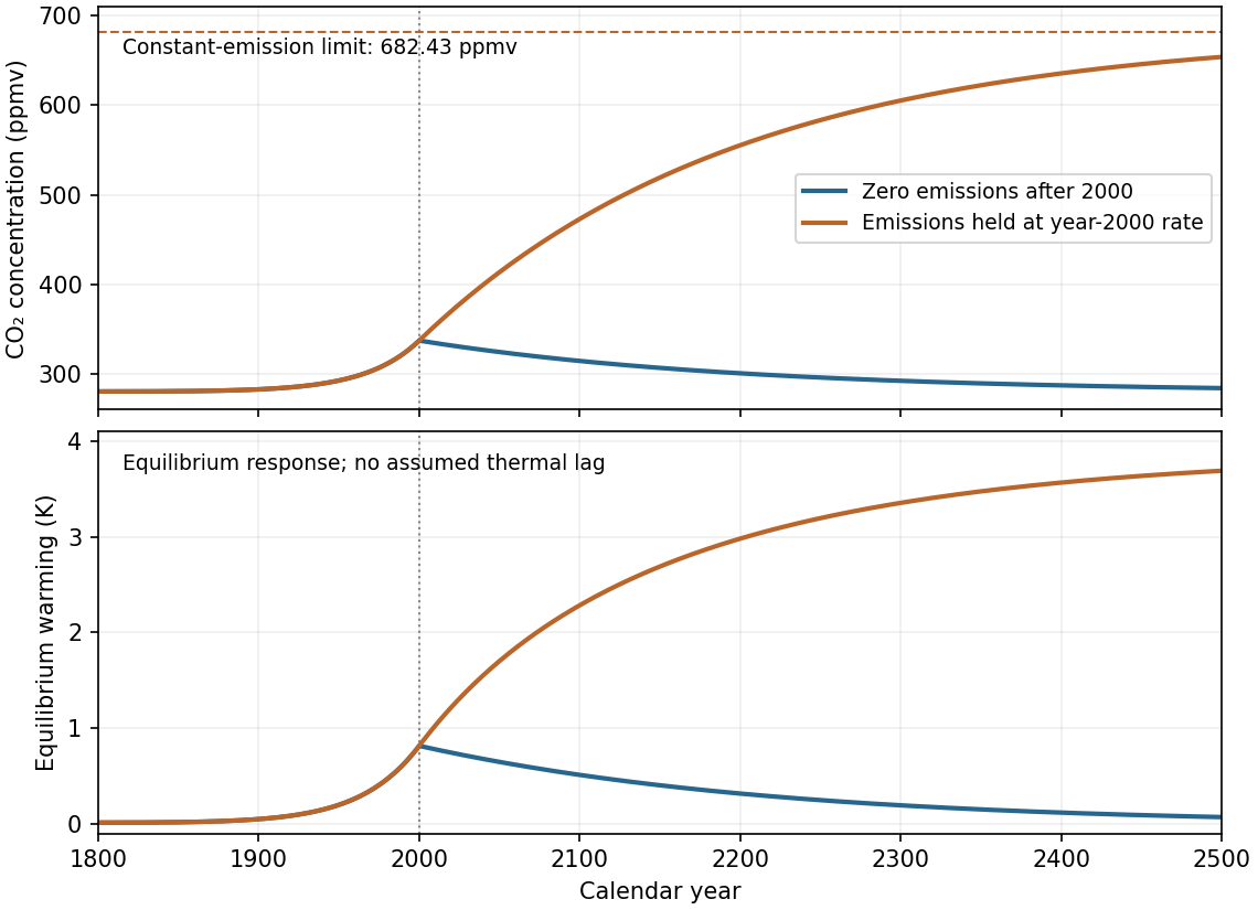
Let $t=0$ now denote the year 2000 and $C_{00}=336.95\mathrm{ppmv}$. When emissions stop, the model givesThe concentration peaks at the switch, then returns exponentially to $279\mathrm{ppmv}$; in 2500 it is about $283.76\mathrm{ppmv}$. Before 2000 both scenarios share the exponential-emissions trajectory.

Using the specified logarithmic equilibrium warming relative to $C_0$,gives the fast-adjustment peak estimateAn unspecified finite thermal response time below twenty years delays and reduces that peak relative to the instantaneous-equilibrium value; its exact amount cannot be fixed without a response law and a chosen thermal time. The carbon-removal time is much longer, so the warming subsequently declines gradually in this model. Taking the 1800 concentration $280$ as the temperature reference instead changes the quoted estimate by only $0.016\mathrm{K}$.

Holding emissions at $E_{00}=8.069\mathrm{GtC}\mathrm{y}{\mathrm{r}}^{-1}$ gives equilibrium concentrationFor time $t$ since 2000,It increases monotonically on the same 200-year timescale and reaches about $654.07\mathrm{ppmv}$ in 2500. The limiting, and hence peak asymptotic, warming isIn 2500 the equilibrium warming is about $3.69\mathrm{K}$, still below that asymptote. A stable thermal adjustment much faster than the carbon timescale follows this slow approach with a short lag and has the same limiting warming. These are predictions of the specified linear reservoir model, not a claim that constant real emissions produce a finite universal atmospheric equilibrium.