Unlettered requests are numbered in source order; explicit letters and Roman parts are retained.
The Laurent series isIts principal part contains infinitely many nonzero negative powers, so zero is an essential singularity. The first three displayed terms are not an asymptotic truncation as z→0; they are the beginning of the convergent Laurent series in powers of 1/z.
e−1/z=∑n=0∞n!(−1)nz−n=1−z1+2z21−6z31+⋯,z=0.
The coefficient of z−1 in the Laurent series is −1. The residue theorem therefore gives, for the standard positive orientation,The residue theorem applies to an isolated essential singularity as well as to a pole.
∮Ce−1/zdz=2πiResz=0e−1/z=−2πi.
Parametrize the positively oriented unit circle by z=eiθ. Then e−1/z=e−cosθ+isinθ and dz=ieiθdθ, soEquating the real part and imaginary part with −2πi gives
∮Ce−1/zdz=i∫02πe−cosθcos(θ+sinθ)dθ−∫02πe−cosθsin(θ+sinθ)dθ.
∫02πe−cosθcos(θ+sinθ)dθ=−2π,∫02πe−cosθsin(θ+sinθ)dθ=0.
The Joukowski map f(z)=z+z−1 is holomorphic on C∖{0}. A holomorphic function is locally conformal where its derivative is nonzero. Here f′(z)=1−z−2 vanishes at z=±1. Thereforewhere the exclusion of zero is because the function is undefined there. Holomorphy alone does not supply conformality at the two critical points.
holomorphic on C∖{0};conformal at every point except 0,1,−1,
Put z=1+ζ. Expanding the holomorphic function near its critical point givesFor a small ray ζ=reiθ, the leading image displacement is r2e2iθ. Thus oriented ray angles are doubled modulo 2π at z=1. This is angle multiplication at a holomorphic critical point of multiplicity two; an unoriented angle between full tangent lines must also be interpreted modulo π. The map is not locally one-to-one there.
f(1+ζ)=2+ζ2−ζ3+O(ζ4).
For z=eiθ the image is w=2cosθ, a real number. Therefore each semicircle maps onto the real interval [−2,2], with endpoints included for closed semicircles. Under positive traversal of the full unit circle, the upper half runs from 2 to −2 and the lower half returns from −2 to 2. Every interior point has two unit-circle preimages. The Joukowski circle-to-ellipse mapping degenerates to a doubled line segment at this radius.
For a radius ρ>0, write z=ρeiθ. ThenFor ρ=1 its image is the ellipseIts horizontal semiaxis is ρ+ρ−1, its vertical semiaxis is ∣ρ−ρ−1∣, and its foci are ±2 because the squared semiaxes differ by 4. Reciprocal radii give the same ellipse, traversed in opposite directions as θ increases.
w=(ρ+ρ−1)cosθ+i(ρ−ρ−1)sinθ.
(ρ+ρ−1)2(Rew)2+(ρ−ρ−1)2(Imw)2=1.
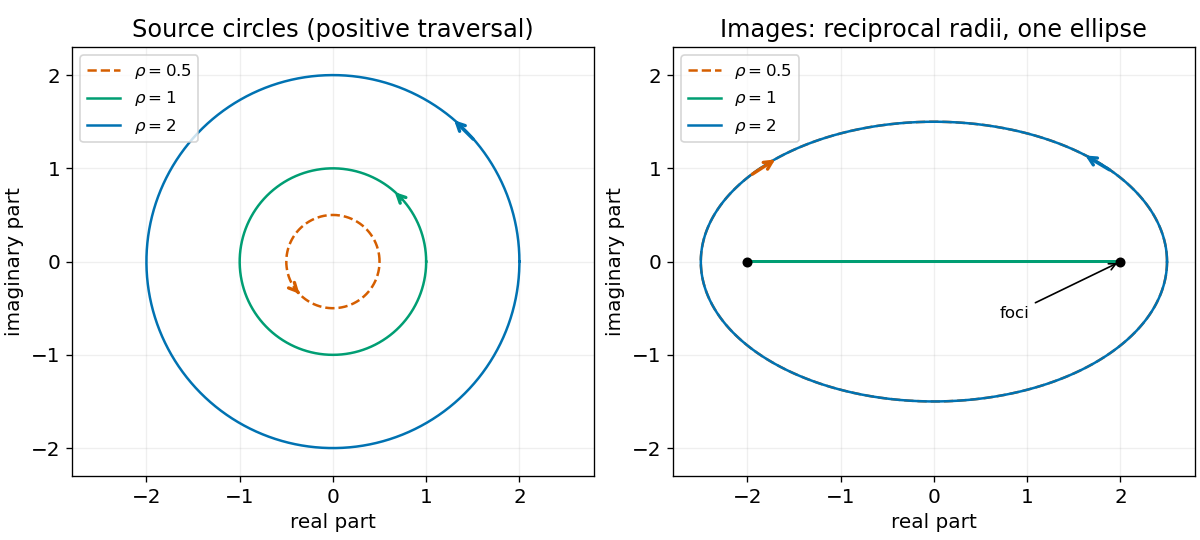
The Joukowski map sends reciprocal-radius circles to one ellipse and the unit circle to a doubled interval
. Details. The square-root branch points are zero and infinity. At zero the local behavior is z−1/2; in the coordinate u=1/z near infinity it is u1/2. In either case one circuit reverses the sign and two restore it. Thus the ramification index is 2: these are two-sheeted algebraic branch points, sometimes described as branch order one when order means ramification index minus one. The decay to zero at infinity does not remove the branching.
TODO: the original closed-contour drawing is absent from the source. The following independent Bromwich contour deformation establishes the required discontinuity relation without asserting the missing drawing's exact geometry. Orient the vertical line upward, as required by the positive imaginary answer in the next part, and use the principal square root, −π<argz<π.
Close a truncated vertical line to the left with a rectangle, slit it along the negative real axis, and exclude a small circle about zero. The integrand is holomorphic inside that slit domain, so the boundary contour integral is zero. Horizontal boundary integrals are O(R−1/2): integrating ex along −R≤x≤1 gives a bounded factor while ∣z∣−1/2≤R−1/2. The left boundary contributes O(e−RR1/2), and the small circle contributes O(ε). All vanish in the indicated limits.
At z=−x with x>0, the upper and lower bank values are respectively −ie−x/x and +ie−x/x. The boundary follows the upper bank toward zero and the lower bank away from zero. Their combined contribution is −2i∫0∞e−xx−1/2dx. HenceThe vertically improper integral converges conditionally; these estimates also justify the contour limit. Reversing the vertical orientation reverses its sign.
I=2i∫0∞e−xx−1/2dx.
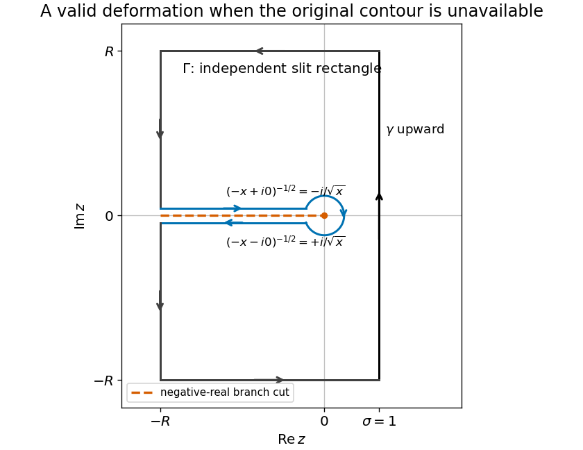
An independently chosen slit-rectangle contour relates the upward Bromwich integral to the square-root branch jump
. Details. The Gamma function identity Γ(1/2)=π gives the Bromwich integral of an inverse square root directly:Equivalently, put x=u2 in the real integral. It becomes 2∫0∞e−u2du=π by the Gaussian integral.
I=2iΓ(1/2)=2iπ.
For two bodies of masses M1,M2, the relative Kepler orbit has semimajor axis a and orbital period P satisfying Kepler's third lawHere a is the semimajor axis of the separation vector, not either star's individual barycentric orbit. In conventional stellar units the same relation is approximately (P/yr)2=(a/AU)3/[(M1+M2)/M⊙], with year, astronomical unit and solar mass as the units.
P2=G(M1+M2)4π2a3.
Equal radial velocity amplitudes imply equal stellar masses. Under the circular, edge-on eclipsing binary interpretation, each star moves at K=100kms−1, and the relative speed is 2K. ThusUsing P=5.45 days givesMore generally, spectroscopic binary amplitudes determine asini=P(K1+K2)1−e2/(2π) and (M1+M2)sin3i=P(K1+K2)3(1−e2)3/2/(2πG). Thus these numerical masses and separation use e=0, sini=1; eclipses alone imply high inclination rather than its exact value.
a=2π(K1+K2)P=1.499×10¹⁰m,M1+M2=2πGP(K1+K2)3.
a≃0.100AU,M1=M2≃2.26M⊙.
TODO: the source light curve, its numerical contact phases and the meanings of the four plotted time labels are absent, so unique numerical stellar radii cannot be recovered. The central eclipse contact-radius relations explain what the missing measurements would determine.
If t1,…,t4 denote the usual first through fourth contacts of a central eclipse, define T14=t4−t1 and T23=t3−t2, and let RL≥RS be the two radii. For a circular edge-on orbit,Taking half their sum and difference gives the radii. For short eclipses the familiar approximation is RL≃vrel(T14+T23)/4 and RS≃vrel(T14−T23)/4, with vrel=2K. At first and fourth contact the discs touch externally; at second and third the smaller disc is just internally tangent to the larger. Noncentral eclipses require the projected impact parameter as well.
RL+RS=asinPπT14,RL−RS=asinPπT23.
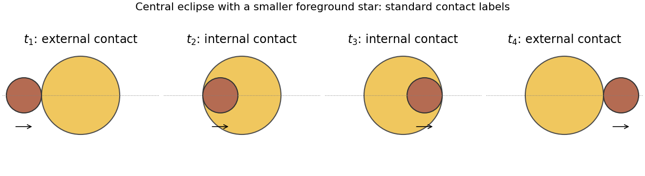
Conditional central-eclipse contact geometry; this schematic supplies no readings from the missing source light curve
. Details. Build the star by adding spherical shells. With m(r) the enclosed mass, its gravitational binding energy isFor a nondegenerate extended star, r(m)<R⊙ on the interior, soThis is a gravitational binding-energy lower bound for a spherical star. The Kelvin-Helmholtz cooling time is of orderThe displayed energy bound gives ∣Ω∣/L⊙>1.6×107 years; it supplies a lower bound on that reservoir-to-luminosity ratio. A stellar structure model sets its coefficient. For an ideal monatomic, gas-supported star the virial theorem puts about half the released gravitational energy into heat, leaving half available for radiation; a uniform-density model would give about 9×10⁶ years. These contraction estimates are all of order 107 years, much shorter than the nuclear lifetime.
Ω=−∫0M⊙r(m)Gmdm.
∣Ω∣>R⊙G∫0M⊙mdm=2R⊙GM⊙2.
τKH∼R⊙L⊙GM⊙2≃3.1×10⁷yr.
Use the supplied atomic masses consistently. Their mass defect per four hydrogen atoms is 4(1.0078)−4.0026=0.0286 atomic mass units. The conversion efficiency isThe atomic-mass bookkeeping includes the associated positron-annihilation energy; an exact photon-heating budget also subtracts energy carried away by neutrinos. With the stated ten-percent fuel fraction and constant present solar luminosity, the main sequence lifetime estimate isThe much longer timescale explains why stellar nuclear fusion can power the Sun throughout its long main-sequence history.
ϵ=4mH4mH−mHe=0.007095≃0.71%.
τMS≃L⊙0.1ϵM⊙c2≃1.05×10¹⁰yr.
A Hertzsprung-Russell diagram plots stellar luminosity upward and effective temperature increasing toward the left. The main sequence runs from hot luminous stars at upper left to cool faint stars at lower right, with the Sun near Teff≃5800K, L=L⊙.
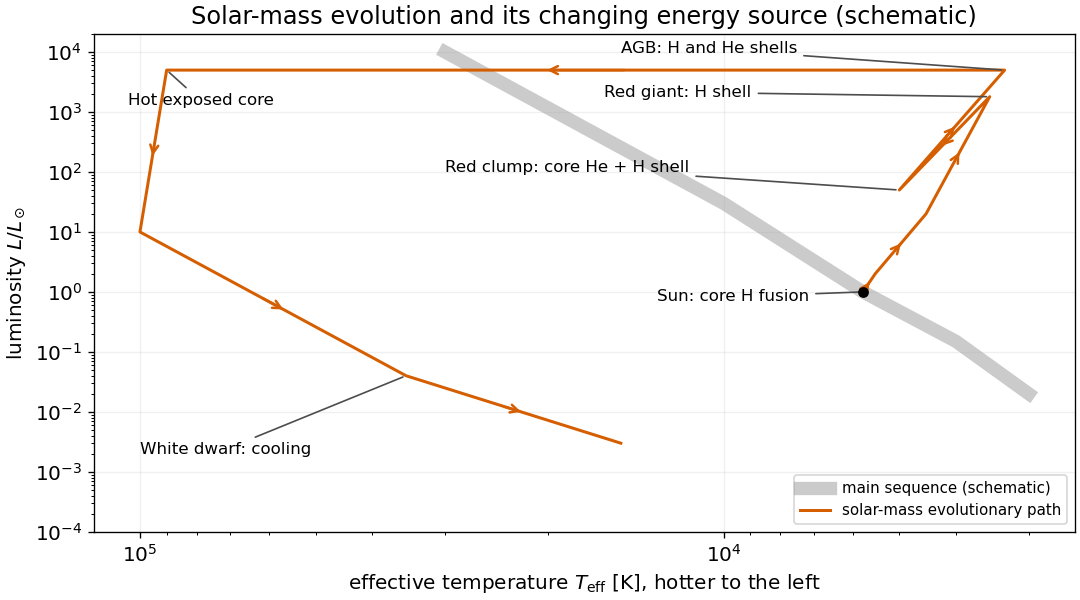
In the evolution of a solar-mass star, core hydrogen fusion initially supplies the luminosity. As core hydrogen is exhausted, hydrogen-shell fusion around a contracting helium core carries the star through the subgiant and red giant phases toward higher luminosity and lower surface temperature. Helium ignition is followed by core helium fusion with a hydrogen-burning shell, placing a solar-mass star in the red clump. The later Asymptotic giant branch has hydrogen- and helium-burning shells around a carbon-oxygen core. Envelope ejection exposes a hot central star of a planetary nebula; residual shell burning ends and the resulting white dwarf radiates stored thermal energy as it cools.


Thermal interstellar dust produces a bright galactic foreground concentrated toward the Milky Way plane, with additional cloud structure. Its emission spectrum differs from the approximately 2.73K blackbody spectrum of the cosmic microwave background, so comparisons across frequencies help separate it. In the sketch below this is the bright equatorial band.
Observer motion produces the cosmic microwave background dipole: to first order in β=v/c,The direction of motion is hotter and the opposite direction cooler. Its full-sky pattern has one broad positive hemisphere and one broad negative hemisphere; it is not concentrated in the galactic plane.
T0ΔT(θ)=βcosθ.
After subtracting the mean, the motion-induced dipole and galactic foregrounds, intrinsic Cosmic microwave background anisotropy appears as angular hot and cold patches, typically at the 10−5 fractional scale. These spatial temperature fluctuations encode early density and velocity structure. The displayed patch pattern is illustrative, with no claim to reproduce an observed sky map.
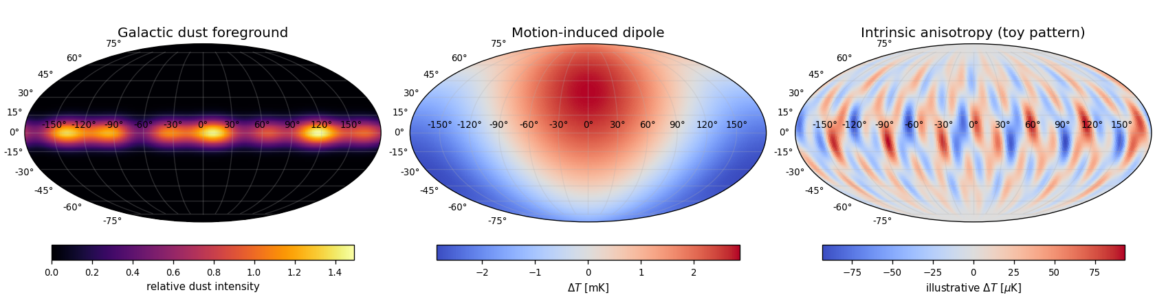
Schematic microwave components: Galactic dust, a kinematic dipole and intrinsic anisotropy, using separate colour scales
. Details. 
Measure the absolute spectral radiance over a range of frequencies and fit the Planck spectrumFor example, the COBE FIRAS blackbody spectrum experiment used a differential Michelson interferometer to compare the sky with an internal blackbody; an external calibrated blackbody could cover the sky entrance. Cold bolometers measured the difference spectrum, and foreground separation distinguished Milky Way emission from the nearly isotropic background. The fitted background temperature is approximately T0=2.73K.[ref]
Bν(T)=c22hν3ehν/(kBT)−11.
The COBE Far Infrared Absolute Spectrophotometer by NASA LAMBDA. Instrument overview: differential internal reference, external calibrator and absolute CMB temperature
The result relies on an absolute spectral comparison, rather than merely measuring a map's hot-to-cold contrast.The stated one-sided temperature contrast is β=0.00105, so the Doppler dipole givesThe motion is toward the hotter region. The contrast already gives one side relative to the mean; the hot-to-cold difference would be twice as large.
v=0.00105c≃3.15×10⁵ms−1=315kms−1.
Adiabatic expansion preserves the blackbody form while each photon's energy redshifts as a−1. Thus the cosmic microwave background temperature obeys T(z)=T0(1+z), giving
T(z=3)=4T0≃10.9K.
Convert both inputs to energy density. The matter contribution, including rest energy, is uM,0=ρM,0c2=2.25×10⁻¹⁰Jm−3. The given photon value is uγ,0=5×10⁵(1.602×10⁻¹⁹)=8.01×10⁻¹⁴Jm−3. HenceMatter energy density scales as (1+z)3, whereas the cosmic microwave background scales as (1+z)4. The photon-only matter-radiation equality condition is thereforeThis uses the supplied CMB photon density. Additional relativistic species change equality for total radiation.
uγ,0uM,0≃2.80×10³.
1+zeq=uγ,0uM,0,zeq≃2.8×10³.
Black-body radiation and the photoelectric effect exposed failures of classical continuous-wave energy exchange. Classical equipartition predicted an unbounded short-wavelength thermal spectrum, the ultraviolet catastrophe. Quantized oscillator energies En=nhν give the mean excitation energy hν/(ehν/(kBT)−1) and suppress high-frequency modes, producing Planck's law. In the modern description, thermal radiation consists of photons with energy hν and Bose occupation numbers.
For the photoelectric effect, increasing intensity below a threshold frequency does not eject electrons, whereas the maximum electron kinetic energy grows with frequency above threshold. Absorption of one photon transfers hν to one electron, giving Kmax=hν−W and threshold ν0=W/h, where W is the work function. Intensity primarily changes the photon arrival rate and hence the photocurrent in the ordinary single-photon regime. Thus changing energy per quantum and changing the number of quanta have distinct consequences. Historically the thermal derivation first quantized matter's energy exchange; it should not be described as an already complete derivation of modern photon theory.
For a photon, pγ=E/c and λγ=hc/E. The neutron is nonrelativistic here because 18.8keV≪mnc2, so pn=2mnE and λn=h/pn. Using the supplied common energy givesEqual kinetic energies do not imply equal momenta: the massive particle obeys E=p2/(2mn), while the massless photon obeys E=pc. The neutron momentum is about 316 times larger, so its de Broglie wavelength is about 316 times smaller.
pγ=1.005×10⁻²³kgms−1,λγ=6.595×10⁻¹¹m,
pn=3.176×10⁻²¹kgms−1,λn=2.086×10⁻¹³m.
To give the neutron the photon wavelength, set its momentum to E/c, not its kinetic energy to E again. ThenIts kinetic energy would then be about 0.188eV, connecting this comparison with the next calculation.
vn≃mncE=5.999×10³ms−1.
For a transverse periodic row of scatterers of spacing d, normal incidence makes their incident phases equal. Scattering at angle θ from that normal creates an outgoing path difference dsinθ between neighbours. Constructive interference requires a phase difference 2πn, givingUsing this printed relation as the intended transverse diffraction grating model, the nonrelativistic neutron wavelength at 0.188eV is λ=6.5964×10⁻¹¹m. Hence the first-order data giveGeometry qualification: this is not a derivation from reflection at crystal planes parallel to the surface, as the source prose says. The ordinary Bragg's law for planes of normal separation d is 2dsinθB=nλ, where θB is the incident glancing angle to those planes. At normal incidence on parallel planes, θB=π/2 and specular reflected rays leave along the normal, so their angle from the normal is zero; they cannot obey the printed positive-order relation dsin0=nλ for λ>0. This is a concrete counterexample to identifying the two geometries. The numerical spacing above is therefore conditional on the printed grating-like relation, rather than a forced assertion that the stated Bragg geometry proves it.
dsinθ=nλ.
d=sin(0.117)λ=5.651×10⁻¹⁰m.
For nonrelativistic neutrons, λ∝EK−1/2, so first-order uncertainty propagation gives ∣Δλ∣/λ=21∣ΔEK∣/EK=0.05. ThusAt fixed d, differentiating the stipulated first-order relation dsinθ=λ gives Δθ=tanθΔλ/λ. ConsequentlyFor photons, λ∝E−1, so the same fractional energy uncertainty gives Δλγ/λγ=0.10. Their 18.8keV wavelength almost equals the low-energy neutron wavelength, so the conditional central angle is 0.116973rad andabout twice the neutron angular spread. This difference comes from the different energy-momentum relations, not from substantially different central wavelengths. The small-angle approximation is adequate at 0.117rad: replacing sinθ by θ changes it by about θ2/6=0.23%, and replacing tanθ by θ changes the sensitivity by about 0.46%. The numerical angular results retain the preceding geometry qualification; a different physical scattering geometry would require its own angle convention.
Δλn≃3.30×10⁻¹²m.
Δθn≃0.00588rad.
Δθγ≃0.01175rad,
In the Franck-Hertz experiment, electrons emitted from a heated cathode are accelerated through a dilute atomic vapour toward a collector. A small retarding potential before the collector rejects electrons that have lost too much kinetic energy. Below the first excitation threshold, mainly elastic collisions occur and the collector current rises as the accelerating voltage increases. At threshold an inelastic collision can transfer a definite excitation energy to an atom, causing a current drop because the slowed electron cannot overcome the retarding potential.
Raising the voltage further permits acceleration again, and repeated losses produce successive current minima. For mercury their spacing is about 4.9V, corresponding to an atomic excitation of about 4.9eV and an associated ultraviolet photon near 254nm. Contact potentials shift the absolute voltages, so the spacing is more informative than the first minimum's position alone. Discrete energy losses support discrete atomic energy levels; a continuously variable excitation energy would not produce the same recurring fixed loss scale. The experiment establishes quantized excitations without requiring the classical electron orbit of the Bohr model to be literally correct.
A classical orbiting electron accelerates and therefore radiates according to the Larmor formula. Its mechanical energy becomes more negative, its radius decreases, and the orbit spirals inward rather than remaining a stable atom. The Bohr model replaces this prediction with postulated nonradiating stationary states and quantized orbital angular momentum, together with photon emission or absorption only between states, hν=∣En−Em∣.
For a heavy nucleus, mevr=nℏ. Since the de Broglie wavelength is h/(mev), this impliesThe electronic wave fits an integer number of wavelengths around the orbit. This is a standing-wave consistency interpretation of the quantization rule, not a classical mechanism that prevents an accelerating charge from radiating. For finite nuclear mass, the two-body relative coordinate uses reduced mass μ=meM/(me+M); the next derivation retains that correction. In the limit M≫me, it reduces to the fixed-nucleus electron description above.
2πr=nλ,n=1,2,….
Let r be the electron-nucleus separation and use the reduced mass μ=meM/(me+M). Coulomb attraction supplies the relative centripetal force, and Bohr quantization fixes the relative angular momentum:Eliminating v givesThe total energy is E=μv2/2−Ze2/(4πϵ0r)=−Ze2/(8πϵ0r), henceHere a0 is the ordinary Bohr radius and R∞ the infinite-nuclear-mass Rydberg constant. The electron's radius about the centre of mass is Mrn/(M+me); for a heavy nucleus this distinction and the reduced-mass correction are small, but the supplied nuclear mass permits them to be stated precisely.
rμv2=4πϵ0r2Ze2,μvr=nℏ.
rn=μZe24πϵ0ℏ2n2=a0μmeZn2.
En=−2(4πϵ0)2ℏ2n2μZ2e4=−hcRMn2Z2,RM=R∞meμ.
The emitted photon carries the decrease in atomic energy, so hc/λ=En−Em for n>m. Using the preceding energy levels givesThe lower state's energy is more negative, making the right-hand side positive. This is the hydrogenic Rydberg formula, with the finite-nuclear-mass factor included in RM.
λ1=RMZ2(m21−n21).
At room temperature, kBT is of order 0.026eV, far smaller than the electronic excitation gaps of the inferred hydrogenic ion. Ground-state absorption is therefore the natural interpretation. Assign the three lines to 1→2, 1→3, and 1→4. Dividing each reciprocal wavelength by its corresponding factor 1−1/n2 givesThe small scatter is consistent with the rounded wavelength data. Since R∞≃1.0974×10⁷m−1 and μ≃me,The ion is thus hydrogen-like lithium, Li2+. If “effective Rydberg constant” denotes only the reduced-mass constant rather than the charge-inclusive spectral coefficient, its value is RM≃Reff/9≃1.097×107m−1. The two conventions are explicitly distinguished; the rounded lines do not determine a precise isotope mass.
Reff=RMZ2≃(9.8765,9.8684,9.8765)×107m−1.
Reff≃9.87×10⁷m−1,Z≃Reff/R∞=3.
For Coulomb binding, the virial theorem gives a typical kinetic energy of the order of the binding energy. Taking ptyp≃2me∣E1∣ and using the Heisenberg uncertainty relation estimate rtyp∼ℏ/ptyp givesThe Bohr model gives r1=a0/Z=a0/2=2.65×10−11m for a heavy helium nucleus, agreeing with the characteristic scale. Equivalently, minimizing the localization estimate E(r)∼ℏ2/(2mer2)−Ze2/(4πϵ0r) gives that same scale.
rtyp∼2me(54.4eV)ℏ=2.65×10⁻¹¹m.
This is an order-of-magnitude radius estimate, not an exact deduction of the cloud's expected value from the inequality alone. Numerical coefficients depend on which spread is used; ΔxΔp≥ℏ/2 does not assert ⟨r⟩=ℏ/p. For the exact hydrogenic 1s state, ⟨r⟩=3a0/(2Z)=3.97×10−11m at Z=2, one and a half times the Bohr orbital radius. An electron cloud has a radial distribution, whereas the Bohr model assigns a definite radius.
The one-dimensional time-independent Schrödinger equation isThe differential term is the kinetic energy operator acting on the wave function, V(x) supplies the multiplicative potential energy, and their sum is the Hamiltonian operator. The eigenvalue E is the stationary state's total energy. This form assumes a nonrelativistic particle, a time-independent scalar potential, and no additional internal degrees of freedom in the stated model.
−2mℏ2dx2d2ψ+V(x)ψ(x)=Eψ(x).
The wave function is a probability amplitude: by the Born rule, ∣ψ(x)∣2dx is the probability of a position measurement in an interval of width dx. For a normalized bound state ∫∣ψ∣2dx=1, the expected values areThe integrals run over the allowed domain. If the given state is not normalized, divide both by ∫∣ψ∣2dx. Its variance is ⟨x2⟩−⟨x⟩2; neither ψ itself nor its overall phase is a directly measured position probability.
⟨x⟩=∫x∣ψ(x)∣2dx,⟨x2⟩=∫x2∣ψ(x)∣2dx.
Each energy eigenstate acquires its own phase under the time-independent Hamiltonian operator:Orthonormality removes all off-diagonal terms from the expected value of the energy, givingReturn up to an overall phase requires the relative phase to return to one. For E1=E2, the shortest positive recurrence time isIf the two energies coincide, the whole superposition is stationary up to a common phase for every time; there is then no smallest strictly positive recurrence time. A half-period changes the relative sign and produces the orthogonal antisymmetric state rather than the original symmetric state.
∣ψ(t)⟩=2e−iE1t/ℏ∣1⟩+e−iE2t/ℏ∣2⟩.
⟨E⟩=2E1+E2,independent of time.
τ=∣E2−E1∣2πℏ.
Projection onto the antisymmetric quantum superposition gives amplitude 21(e−iE1t/ℏ−e−iE2t/ℏ). Its squared modulus isIt vanishes initially, reaches one at a half-recurrence time, and returns to zero after τ. This interference depends on a relative phase even though each energy-eigenstate population and the mean energy remain constant.
P+→−(t)=sin2(2ℏ(E2−E1)t).
An ideal projective measurement yielding the antisymmetric state prepares that state at t1. Starting from it, the probability of reaching the symmetric state after an additional interval s is again sin2((E2−E1)s/(2ℏ)). At the full recurrence interval found above,The full-period propagator is proportional to the identity on the two-dimensional subspace, so it returns the antisymmetric state to itself, not to its orthogonal partner. The result assumes the stated time-independent evolution continues after the measurement.
P(+ at t1+τ∣− at t1)=sin2π=0.
Choose the infinite well as 0<x<a with real eigenfunctions ψn=2/asin(nπx/a). This fixes the relative phase convention for the specified initial plus state. Each of the first two states has probability 1/2 in the left half. Their cross integral isThe evolving superposition therefore givesSince En=n2π2ℏ2/(2ma2), the angular frequency and ordinary frequency areThe probability varies between 1/2±4/(3π) and remains in [0,1]. Changing the sign convention of one eigenfunction while keeping the same physical initial state requires changing its superposition coefficient too; otherwise one has prepared the other initial state and reversed the initial spatial bias.
∫0a/2ψ1ψ2dx=π2∫0π/2sinusin2udu=3π4.
Pleft(t)=21+3π4cos(ℏ(E2−E1)t).
ω=2ma23π2ℏ,f=2πω=8ma23h.
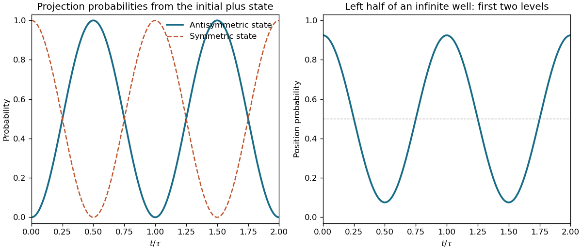
Original two-state transition and left-half well probabilities over two recurrence periods
. Details. 
Annual conversion is reduced by several multiplicative losses. Only roughly 40–50% of incident sunlight lies in the photosynthetically useful visible band. Reflection and transmission prevent complete absorption; the photon budget and unavoidable relaxation losses limit conversion of absorbed radiation into chemical energy. Photosynthesis also has to support respiration and maintenance, while seasonal growth, incomplete canopy cover, water and nutrient limitations reduce the annual harvested yield.
An illustrative loss budget, not a universal biological constant, is 0.45×0.8×0.25×0.5×0.11≃0.005. The factors represent useful spectrum, absorption, photochemical conversion, retained net production, and combined annual interception and growing-condition limitations, respectively. Thus ηannual∼0.5% is plausible for a land-averaged crop yield even though a leaf under favourable illumination can be more efficient. The result depends on crop, climate, harvested fraction and the definition of dry biomass energy. When the input is already annual mean insolation, night-time must not be counted as a second independent loss.
Take an explicitly illustrative European annual mean ground-level irradiance of 100Wm−2, the stated conversion fraction 0.005, and dry carbohydrate heating value 16MJkg−1. One square kilometre then producesHence M∼103tonneskm−2year−1, or about 10tonnesha−1year−1, as a dry-mass order-of-magnitude estimate. The assumed irradiance is not a site-specific value supplied by the paper. The result scales linearly with irradiance and conversion efficiency and inversely with heating value; wet harvested mass would additionally depend on water content.
M=16×106(100)(106)(3.156×10⁷)(0.005)=9.86×10⁵kgyear−1.
Use equal combustion energy as the displacement criterion. The petrol mass and energy areThis needs ethanol mass Me=Qp/(30.5×106)=1.04115×1010kg. The ethanol fermentation stoichiometry converts 180 mass units of glucose to 92 of ethanol, so the ethanol yield per square kilometre is (1500)(92/180)=766.667 tonnes. ThereforeThe carbon mass fraction in octane is 8(12)/(8(12)+18)=96/114. The displaced fossil carbon is thusThis is the ideal net reduction if the crop regrows and its carbon dioxide uptake balances the biogenic carbon released in fermentation and combustion, with negligible additional life-cycle emissions. Ethanol combustion is not carbon-free: it releases about 5.43 million tonnes of carbon here, and fermentation releases further biogenic carbon. Those are balanced by crop uptake in the stated ideal accounting, rather than being ignored. Farming, fertilizer manufacture, processing heat, transport and land-use carbon losses reduce the actual benefit and may even reverse it. The equal-heat calculation also assumes equal useful-energy conversion efficiencies in the displaced application; it does not establish equal engine mileage automatically.
Mp=0.73(1010)=7.3×10⁹kg,Qp=Mp(43.5×10⁶)=3.1755×10¹⁷J.
A=766.6671.04115×107≃1.358×10⁴km2.
ΔMC,fossil=7.3×1091149610001=6.15×10⁶tonnes Cyear−1.
Three advantages of biomass energy are:
- Sustainable regrowth can replenish the fuel and recycle its biogenic carbon, unlike depletion of fossil carbon stocks.
- Chemical fuel can be stored and transported, permitting dispatchable heat, electricity or liquid-fuel production rather than requiring use at the instant of sunlight capture.
- Suitable agricultural residues and organic wastes can supply useful energy while recovering value from material that would otherwise need disposal.
Three disadvantages are:
- Dedicated energy crops compete for land and water, potentially displacing food production and damaging biodiversity.
- Low annual areal productivity, bulky feedstock and moisture increase collection, transport, drying and conversion costs.
- Combustion produces local air pollutants, and processing emissions or land-use carbon debt can undermine the claimed climate saving. A life-cycle assessment and a regrowth timescale are necessary; “renewable” alone does not prove low net emissions.
Articles were limited to the first 100 out of 370 total.
Ancestors (8)
- Past exam of the short options paper shared by Prelims and Parts A and B of the physics course of the University of Oxford
- Short options paper shared by Prelims and Parts A and B of the physics course of the University of Oxford
- Physics course of the University of Oxford
- Undergraduate course of the University of Oxford
- Course of the University of Oxford
- University of Oxford
- List of universities
- Home
Discussion (0)
New discussionThere are no discussions about this article yet.
Articles by others on the same topic (0)
There are currently no matching articles.