Complete oxidation of 1012kg of carbon adds nC=1012/(12×10−3)=8.33×1013mol of carbon dioxide. With atmospheric mass about 5.1×10¹⁸kg and mean air molar mass 28.97×10⁻³kgmol−1, there are about 1.76×10²⁰mol of air. The dry-air mole fraction, approximately the volume fraction, changes byIt is the carbon inventory that counts: oxidation adds oxygen to each molecule but does not change the number of carbon-containing molecules. Using 5.15×10¹⁸kg instead changes the estimate by only about one percent. The atmospheric constants are standard Earth estimates, not additional data read from a missing plot.[ref]
ΔC≃1061.76×10208.33×1013≃0.47ppmv per GtC.
The term b1E is the effective atmospheric addition from ongoing emissions. Its coefficient 0.25ppmv/GtC is about half the full-retention estimate 0.47ppmv/GtC, so the model implicitly removes or partitions some emitted carbon promptly. The term −b0(C−C0) represents slower net uptake of the excess by other reservoirs; its relaxation time is b0−1=200 years. Both terms have units of ppmv per year.
Thousands of years at constant E0 erase the initial transient, givingThe reference C0 is the zero-anthropogenic-emission equilibrium, not the equilibrium when the stated small persistent emissions are present.
0=b1E0−b0(C−C0),C(1800)=C0+b0b1E0=279+1=280ppmv.
Put A=b1E0/b0. The proposed solution can be writtenIt gives C(0)−C0=A. Differentiation and substitution give, respectively,so it satisfies both the differential equation and the initial condition. At t=200 years,with E(2000)=0.02e6≃8.069GtCyr−1. The earlier emissions grow on the g−1=33.3 year timescale, much faster than the model's 200-year removal time.
C−C0=g+b0A(ge−b0t+b0egt).
C˙=g+b0Agb0(egt−e−b0t),
b1E0egt−b0(C−C0)=g+b0Agb0(egt−e−b0t),
C(2000)=279+0.0350.03e−1+0.005e6≃336.95ppmv,
Let t=0 now denote the year 2000 and C00=336.95ppmv. When emissions stop, the model givesThe concentration peaks at the switch, then returns exponentially to 279ppmv; in 2500 it is about 283.76ppmv. Before 2000 both scenarios share the exponential-emissions trajectory.
C(t)=C0+(C00−C0)e−t/(200yr).
Using the specified logarithmic equilibrium warming relative to C0,gives the fast-adjustment peak estimateAn unspecified finite thermal response time below twenty years delays and reduces that peak relative to the instantaneous-equilibrium value; its exact amount cannot be fixed without a response law and a chosen thermal time. The carbon-removal time is much longer, so the warming subsequently declines gradually in this model. Taking the 1800 concentration 280 as the temperature reference instead changes the quoted estimate by only 0.016K.
ΔTeq(C)=3log2(C/C0)K,
ΔTpeak≈3log2(336.95/279)≃0.82K.
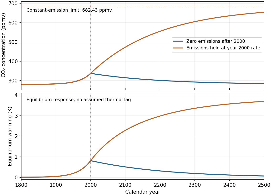
The two specified carbon-emission scenarios from 1800 to 2500
. Both curves share the prescribed emissions growth up to 2000. Zero later emissions give exponential return to 279 ppmv; holding emissions constant gives approach to 682.43 ppmv. The inset-free lower panel shows equilibrium warming rather than an invented thermal adjustment history. Details.
Holding emissions at E00=8.069GtCyr−1 gives equilibrium concentrationFor time t since 2000,It increases monotonically on the same 200-year timescale and reaches about 654.07ppmv in 2500. The limiting, and hence peak asymptotic, warming isIn 2500 the equilibrium warming is about 3.69K, still below that asymptote. A stable thermal adjustment much faster than the carbon timescale follows this slow approach with a short lag and has the same limiting warming. These are predictions of the specified linear reservoir model, not a claim that constant real emissions produce a finite universal atmospheric equilibrium.
C∞=C0+b0b1E00≃682.43ppmv.
C(t)=C∞+(C00−C∞)e−t/(200yr).
ΔTpeak⟶3log2(682.43/279)≃3.87K.
The real carbon cycle has multiple reservoirs and adjustment times, rather than one universally exponential removal process. Air-sea exchange, ocean mixing and carbonate chemistry give a long-lived atmospheric tail; uptake also changes with temperature, circulation and carbon loading. For example, a warming ocean can absorb less additional carbon dioxide, so a fixed b0 omits a potentially positive climate-carbon feedback. Terrestrial vegetation and soil responses provide further examples. One missing feature is the dependence of carbon uptake on the changing state of the ocean and climate.
Ancestors (10)
- S25
- 2012
- Past exam of the short options paper shared by Prelims and Parts A and B of the physics course of the University of Oxford
- Short options paper shared by Prelims and Parts A and B of the physics course of the University of Oxford
- Physics course of the University of Oxford
- Undergraduate course of the University of Oxford
- Course of the University of Oxford
- University of Oxford
- List of universities
- Home
Discussion (0)
New discussionThere are no discussions about this article yet.
Articles by others on the same topic (0)
There are currently no matching articles.