Spectral irradiance Fλ is radiant power crossing unit area per unit wavelength, integrated over the relevant hemisphere with the projected-area factor: Fλ=∫IλcosθdΩ. Its units are Wm−2 per unit wavelength; spectral radiance Iλ additionally refers to unit solid angle. For an isotropic outgoing hemisphere with Planck function Bλ, the integral is Fλ=πBλ.
The vertical optical depth above height z is the dimensionless extinction integralHere z increases upward, na is absorber number density, σλ its absorption cross section, ρa its mass density, and κλ the absorption coefficient per unit absorber mass. Equivalently, using bulk air density ρ and absorber mass fraction qa, dτλ/dz=−κλqaρ. The coefficient may depend on temperature, pressure and wavelength. For purely absorbing gas, transmission along a ray is e−τray; scattering, if present, contributes to extinction and requires its own source term.
τλ(z)=∫z∞na(z′)σλ(z′)dz′,dzdτλ=−naσλ=−κλρa.
Use the optical-depth weighting stipulated in the paper. A jump in the Planck function at τ1 gives dB/dτ=(B1−B0)δ(τ−τ1), soThe upper isothermal layer emits πB0(1−e−τ1) and transmits the lower region's blackbody spectral irradiance with factor e−τ1. The lower layer and black surface have the same B1, so their combined radiation entering the upper layer is πB1, independent of how its emission is divided between the lower gas and surface.
I0=π[B0+(B1−B0)e−τ1]=πB0(1−e−τ1)+πB1e−τ1.
More generally, integration by parts rewrites the supplied expression asThe terms are attenuated surface emission and the atmosphere's own emission. In the original boundary-plus-gradient form, πB0 is the isothermal reference flux and the integral corrects for temperature variation below the top. Optical depths of order unity contribute most strongly. These formulas follow the paper's specified exponential weighting; a full angular radiative transfer calculation uses ray-angle-dependent optical paths rather than identifying every ray with a vertical path.
I0=πB(τs)e−τs+π∫0τsB(τ)e−τdτ.
For the linear Planck function profile, direct integration givesin the optically thick limit. A sudden doubling of absorber abundance doubles optical depth at every physical height while initially leaving the temperature profile fixed. With τ=2τ, the same profile is B=B0+(α/2)τ, not B0+ατ. ThusIf temperature increases downward, α>0 and outgoing spectral irradiance decreases immediately because the effective emitting region moves upward into cooler gas. Subsequent thermal adjustment is outside this instantaneous comparison.
I0=πB0+πα(1−e−τs)⟶π(B0+α)
I0=π(B0+α/2),ΔI0=−2πα.
For the quadratic Planck function profile,The optically thick limit and the instantaneous doubled-abundance result are thereforeThe new coefficient is β/4, since B(τ)=B0+β(τ/2)2 at fixed physical temperature. For positive β, the outgoing spectral irradiance decreases. The factor differs from the linear case because the temperature-dependent source function curves with depth; doubling abundance does not mean holding its old functional coefficients fixed in the new optical-depth coordinate.
I0=πB0+2πβ∫0τsτe−τdτ=πB0+2πβ[1−(1+τs)e−τs].
I0=π(B0+2β),I0=π(B0+β/2),ΔI0=−23πβ.
Hydrostatic equilibrium balances the vertical pressure gradient against weight, dP/dz=−ρg. For a dry ideal gas parcel displaced slowly enough to maintain pressure balance but rapidly enough to exchange negligible heat, the first law givesCombining the two equations yields the dry adiabatic lapse rateusing cp≃1004Jkg−1K−1. Here temperature in the thermodynamic differential is absolute, g and cp are treated as constant, composition is fixed, and condensation is excluded. Hydrostatic balance alone does not force the atmosphere to be adiabatic; the parcel assumption supplies the extra relation.
cpdT−ρ1dP=0.
Γd=−dzdT=cpg≃9.8Kkm−1,
Water condensation releases latent heat, reducing the cooling of a rising saturated parcel and giving a smaller moist adiabatic lapse rate. Radiation, mixing, large-scale motion and incomplete convective adjustment also shape the environmental lapse rate. Thus an observed 6--7Kkm−1 need not equal the dry parcel value and is broadly consistent with a moist, radiatively influenced atmosphere.
Write s=Ts−273.15K as the numerical sea-level Celsius temperature in degrees Celsius, and use the same degree increments for Γz. The model's top temperature is TC=s−Γz. For positive α its intended cold-ice branch has TC<0, so the positive melt-loss magnitude and snow gain areThe model is singular at z=s/Γ and is not a physical melting law across that boundary. On the relevant interval s/Γ<z<1/β, L decreases hyperbolically and A decreases linearly. Assume a fixed area and positive ice density, so increasing mass increases z: stability has the same sign as F′(z).
L(z)=Γz−sα,A(z)=1−βz,F(z)=M˙=A(z)−L(z).
The equilibrium equation iswith rootsTwo distinct physical equilibria, one stable, exist providedThis combines a positive allowed interval with a strictly positive discriminant. At the larger root F′<0 and small perturbations restore the ice cap; the smaller root has F′>0 and is unstable. Sincea restoring local response requiresThis is the lower height bound from the stability derivative; the stable equilibrium itself is z+. The minimum initial height for persistence, a different notion of threshold, is the unstable separator z−: initial heights above it approach z+, while lower heights lose ice and leave the model's cold branch. At equality in the discriminant condition the two equilibria merge, giving a marginal fold rather than a strictly stable ice cap.
(1−βz)(Γz−s)=α,
z±=2βΓΓ+βs±(Γ−βs)2−4αβΓ.
Γ−βs>2αβΓ⟺s<βΓ−2βαΓ.
F′(z)=−β+(Γz−s)2αΓ,
z>zslope=Γs+βΓα.
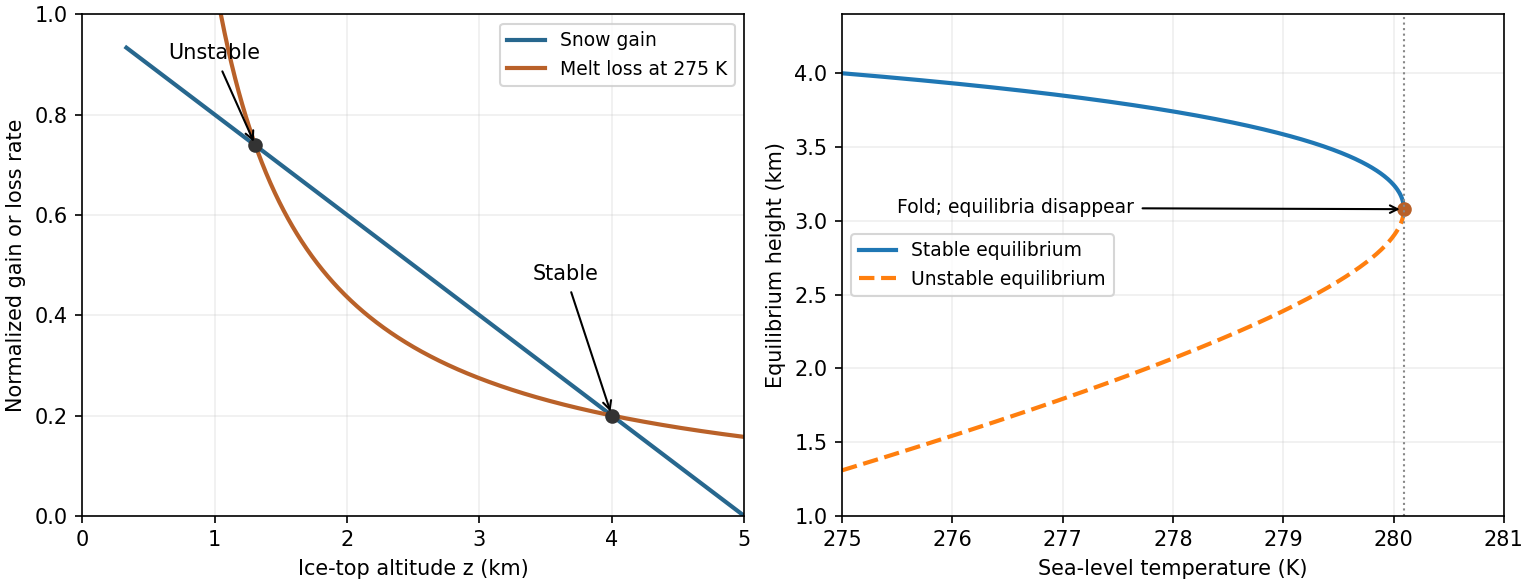

At z=4km, the snow gain is 1−0.2(4)=0.2 and the model's top Celsius temperature is 275−273.15−6(4)=−22.15∘C. Equilibrium givesin the normalized rate convention. Using 273K for the Celsius zero instead would give 4.4∘C. The local slope is −0.2+4.43(6)/(22.15)2≃−0.1458km−1<0, as required. Initially z−=1.3083km and zslope≃2.230km, while z+=4km.
α=0.2(22.15)=4.43∘C
As Ts slowly rises, melt loss increases at fixed z, the stable high branch moves downward and the unstable branch upward. They merge atBeyond the fold the model has no steady cold ice cap: its net balance is negative throughout the physical interval and ice shrinks until the assumed law ceases to apply. Quasistatic tracking presumes adjustment is fast compared with the imposed warming, an assumption that deteriorates near the fold as the restoring slope tends to zero. This singular idealized law is not a quantitative real-world melting forecast.
scrit=0.26−20.24.43(6)≃6.944∘C,
Ts,crit≃280.09K,ΔTs≃5.09K,zfold≃3.079km.
Complete oxidation of 1012kg of carbon adds nC=1012/(12×10−3)=8.33×1013mol of carbon dioxide. With atmospheric mass about 5.1×10¹⁸kg and mean air molar mass 28.97×10⁻³kgmol−1, there are about 1.76×10²⁰mol of air. The dry-air mole fraction, approximately the volume fraction, changes byIt is the carbon inventory that counts: oxidation adds oxygen to each molecule but does not change the number of carbon-containing molecules. Using 5.15×10¹⁸kg instead changes the estimate by only about one percent. The atmospheric constants are standard Earth estimates, not additional data read from a missing plot.[ref]
ΔC≃1061.76×10208.33×1013≃0.47ppmv per GtC.
The term b1E is the effective atmospheric addition from ongoing emissions. Its coefficient 0.25ppmv/GtC is about half the full-retention estimate 0.47ppmv/GtC, so the model implicitly removes or partitions some emitted carbon promptly. The term −b0(C−C0) represents slower net uptake of the excess by other reservoirs; its relaxation time is b0−1=200 years. Both terms have units of ppmv per year.
Thousands of years at constant E0 erase the initial transient, givingThe reference C0 is the zero-anthropogenic-emission equilibrium, not the equilibrium when the stated small persistent emissions are present.
0=b1E0−b0(C−C0),C(1800)=C0+b0b1E0=279+1=280ppmv.
Put A=b1E0/b0. The proposed solution can be writtenIt gives C(0)−C0=A. Differentiation and substitution give, respectively,so it satisfies both the differential equation and the initial condition. At t=200 years,with E(2000)=0.02e6≃8.069GtCyr−1. The earlier emissions grow on the g−1=33.3 year timescale, much faster than the model's 200-year removal time.
C−C0=g+b0A(ge−b0t+b0egt).
C˙=g+b0Agb0(egt−e−b0t),
b1E0egt−b0(C−C0)=g+b0Agb0(egt−e−b0t),
C(2000)=279+0.0350.03e−1+0.005e6≃336.95ppmv,
Let t=0 now denote the year 2000 and C00=336.95ppmv. When emissions stop, the model givesThe concentration peaks at the switch, then returns exponentially to 279ppmv; in 2500 it is about 283.76ppmv. Before 2000 both scenarios share the exponential-emissions trajectory.
C(t)=C0+(C00−C0)e−t/(200yr).
Using the specified logarithmic equilibrium warming relative to C0,gives the fast-adjustment peak estimateAn unspecified finite thermal response time below twenty years delays and reduces that peak relative to the instantaneous-equilibrium value; its exact amount cannot be fixed without a response law and a chosen thermal time. The carbon-removal time is much longer, so the warming subsequently declines gradually in this model. Taking the 1800 concentration 280 as the temperature reference instead changes the quoted estimate by only 0.016K.
ΔTeq(C)=3log2(C/C0)K,
ΔTpeak≈3log2(336.95/279)≃0.82K.
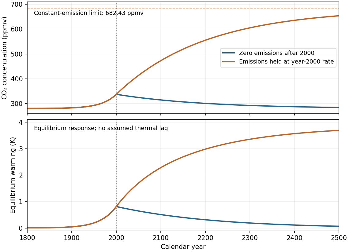
The two specified carbon-emission scenarios from 1800 to 2500
. Both curves share the prescribed emissions growth up to 2000. Zero later emissions give exponential return to 279 ppmv; holding emissions constant gives approach to 682.43 ppmv. The inset-free lower panel shows equilibrium warming rather than an invented thermal adjustment history. Details.
Holding emissions at E00=8.069GtCyr−1 gives equilibrium concentrationFor time t since 2000,It increases monotonically on the same 200-year timescale and reaches about 654.07ppmv in 2500. The limiting, and hence peak asymptotic, warming isIn 2500 the equilibrium warming is about 3.69K, still below that asymptote. A stable thermal adjustment much faster than the carbon timescale follows this slow approach with a short lag and has the same limiting warming. These are predictions of the specified linear reservoir model, not a claim that constant real emissions produce a finite universal atmospheric equilibrium.
C∞=C0+b0b1E00≃682.43ppmv.
C(t)=C∞+(C00−C∞)e−t/(200yr).
ΔTpeak⟶3log2(682.43/279)≃3.87K.
The real carbon cycle has multiple reservoirs and adjustment times, rather than one universally exponential removal process. Air-sea exchange, ocean mixing and carbonate chemistry give a long-lived atmospheric tail; uptake also changes with temperature, circulation and carbon loading. For example, a warming ocean can absorb less additional carbon dioxide, so a fixed b0 omits a potentially positive climate-carbon feedback. Terrestrial vegetation and soil responses provide further examples. One missing feature is the dependence of carbon uptake on the changing state of the ocean and climate.
Ancestors (9)
- 2012
- Past exam of the short options paper shared by Prelims and Parts A and B of the physics course of the University of Oxford
- Short options paper shared by Prelims and Parts A and B of the physics course of the University of Oxford
- Physics course of the University of Oxford
- Undergraduate course of the University of Oxford
- Course of the University of Oxford
- University of Oxford
- List of universities
- Home
Discussion (0)
New discussionThere are no discussions about this article yet.
Articles by others on the same topic (0)
There are currently no matching articles.