Past exam of the short options paper shared by Prelims and Parts A and B of the physics course of the University of Oxford / 2012 / S9 / 1

Stylized facts of financial returns are robust qualitative statistical regularities found across many instruments or datasets, abstracting from their individual details. Examples include heavy return-distribution tails relative to a Gaussian model, weak linear autocorrelation of many liquid-market returns beyond short lags, and persistent clustering of large absolute or squared returns. Some markets also show asymmetric return-volatility responses and partial movement toward a Gaussian aggregate distribution at longer horizons.

These are empirical tendencies with sampling-scale and market qualifications, not exact universal equations. In particular, weak return autocorrelation does not imply independent increments: volatility clustering and higher-order dependence can remain. A useful model should state which regularities it explains and which its assumptions exclude, rather than treating one convenient random-walk model as an observed law.

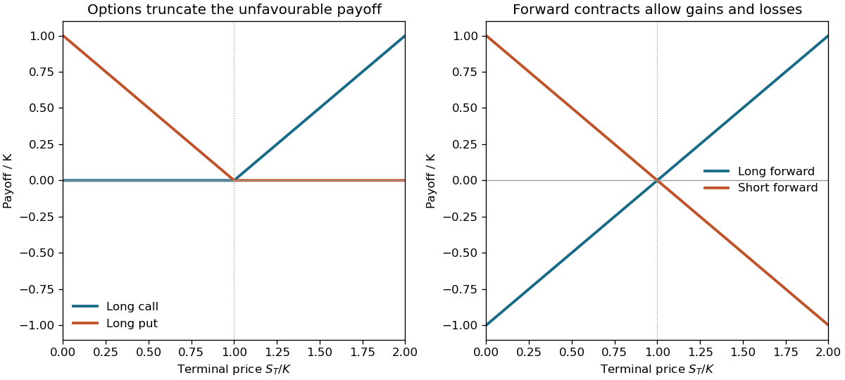
Let $S_T$ be the terminal asset price and $K$ a common strike or forward delivery price. A long European call and put have expiry payoffsThe call is zero below $K$ and then rises with slope one; the put falls with slope minus one below $K$ and is zero above it. A long forward instead has $\boxed{F_T^{\mathrm{long}}=S_T-K}$ and a short forward has $\boxed{F_T^{\mathrm{short}}=K-S_T}$. Both are straight lines crossing zero at $K$, with negative as well as positive outcomes.

The option's exercise right truncates the unfavourable side, whereas the forward is an obligation. These are payoffs, not total profits: an option premium and its financing cost have not been subtracted. A newly agreed fair forward may have zero initial value while still having a nonzero future delivery price.

Assume a non-dividend-paying tradable asset follows geometric Brownian motion $dS=\mu Sdt+\sigma SdW$, with constant volatility $\sigma$ and risk-free rate $r$. Trading is continuous, frictionless and divisible; borrowing and lending occur at the same rate, short selling is allowed, the strategy is self-financing, and there are no jumps or arbitrage opportunities. These are modelling assumptions, not assertions that market returns are exactly Gaussian or that hedging is costless in practice.

For a smooth option price $V(S,t)$, Itô's formula givesReplicate it by $\Delta$ shares and a cash account of value $b=V-\Delta S$. Self-financing requires $dV=\Delta dS+rbdt$. Matching the stochastic term fixes $\Delta =V_S$. Matching the remaining drift and cancelling the physical drift $\mu$ then givesThis is the Black-Scholes equation. The cancellation does not assert that the actual expected asset return equals $r$; risk-neutral valuation is a consequence of replication under these assumptions.

For a European call, impose $V(S,T)=(S-K{)}^{+}$, with $V(0,t)=0$ and $V(S,t)\sim S-K{e}^{-r(T-t)}$ for large $S$. Its writer hedges the short option by holding $\Delta =\partial V/\partial S$ shares and investing or borrowing the residual cash $V-\Delta S$, rebalancing as $S$ and time change. In the constant-parameter model $\Delta =N(d_1)$, where $d_1=[\log (S/K)+(r+{\sigma }^2/2)(T-t)]/[\sigma \sqrt{T-t}]$ and $N$ is the standard normal cumulative distribution. Continuous rebalancing is an ideal limit: transaction costs, discrete trading, jumps and changing volatility create residual hedge risk. Writing the self-financing gains equation explicitly avoids incorrectly adding an unfinanced $Sd\Delta$ term to the strategy.

Implied volatility is the volatility parameter that makes a specified option-pricing model reproduce an observed option price. For a call, it solvesFor positive time to expiry and positive asset and strike prices, the Black-Scholes call price increases with $\sigma$, so an interior arbitrage-consistent price gives a unique finite positive value. It is an inverse model parameter, not the sample standard deviation of past returns or a guaranteed forecast of future realised volatility. Different implied volatilities across strikes or maturities form smiles or surfaces, signalling that one constant volatility does not fit all prices simultaneously.