Past exam of the short options paper shared by Prelims and Parts A and B of the physics course of the University of Oxford / 2012 / S9 (Financial physics)

Stylized facts of financial returns are robust qualitative statistical regularities found across many instruments or datasets, abstracting from their individual details. Examples include heavy return-distribution tails relative to a Gaussian model, weak linear autocorrelation of many liquid-market returns beyond short lags, and persistent clustering of large absolute or squared returns. Some markets also show asymmetric return-volatility responses and partial movement toward a Gaussian aggregate distribution at longer horizons.

These are empirical tendencies with sampling-scale and market qualifications, not exact universal equations. In particular, weak return autocorrelation does not imply independent increments: volatility clustering and higher-order dependence can remain. A useful model should state which regularities it explains and which its assumptions exclude, rather than treating one convenient random-walk model as an observed law.

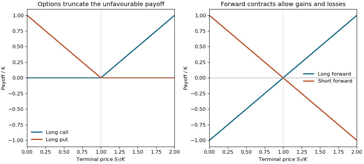
Let $S_T$ be the terminal asset price and $K$ a common strike or forward delivery price. A long European call and put have expiry payoffsThe call is zero below $K$ and then rises with slope one; the put falls with slope minus one below $K$ and is zero above it. A long forward instead has $\boxed{F_T^{\mathrm{long}}=S_T-K}$ and a short forward has $\boxed{F_T^{\mathrm{short}}=K-S_T}$. Both are straight lines crossing zero at $K$, with negative as well as positive outcomes.

The option's exercise right truncates the unfavourable side, whereas the forward is an obligation. These are payoffs, not total profits: an option premium and its financing cost have not been subtracted. A newly agreed fair forward may have zero initial value while still having a nonzero future delivery price.

Assume a non-dividend-paying tradable asset follows geometric Brownian motion $dS=\mu Sdt+\sigma SdW$, with constant volatility $\sigma$ and risk-free rate $r$. Trading is continuous, frictionless and divisible; borrowing and lending occur at the same rate, short selling is allowed, the strategy is self-financing, and there are no jumps or arbitrage opportunities. These are modelling assumptions, not assertions that market returns are exactly Gaussian or that hedging is costless in practice.

For a smooth option price $V(S,t)$, Itô's formula givesReplicate it by $\Delta$ shares and a cash account of value $b=V-\Delta S$. Self-financing requires $dV=\Delta dS+rbdt$. Matching the stochastic term fixes $\Delta =V_S$. Matching the remaining drift and cancelling the physical drift $\mu$ then givesThis is the Black-Scholes equation. The cancellation does not assert that the actual expected asset return equals $r$; risk-neutral valuation is a consequence of replication under these assumptions.

For a European call, impose $V(S,T)=(S-K{)}^{+}$, with $V(0,t)=0$ and $V(S,t)\sim S-K{e}^{-r(T-t)}$ for large $S$. Its writer hedges the short option by holding $\Delta =\partial V/\partial S$ shares and investing or borrowing the residual cash $V-\Delta S$, rebalancing as $S$ and time change. In the constant-parameter model $\Delta =N(d_1)$, where $d_1=[\log (S/K)+(r+{\sigma }^2/2)(T-t)]/[\sigma \sqrt{T-t}]$ and $N$ is the standard normal cumulative distribution. Continuous rebalancing is an ideal limit: transaction costs, discrete trading, jumps and changing volatility create residual hedge risk. Writing the self-financing gains equation explicitly avoids incorrectly adding an unfinanced $Sd\Delta$ term to the strategy.

Implied volatility is the volatility parameter that makes a specified option-pricing model reproduce an observed option price. For a call, it solvesFor positive time to expiry and positive asset and strike prices, the Black-Scholes call price increases with $\sigma$, so an interior arbitrage-consistent price gives a unique finite positive value. It is an inverse model parameter, not the sample standard deviation of past returns or a guaranteed forecast of future realised volatility. Different implied volatilities across strikes or maturities form smiles or surfaces, signalling that one constant volatility does not fit all prices simultaneously.

Independent identically distributed increments have the same marginal distribution at every step and factorizing joint distributions across steps. With finite mean $\mu$ and variance $s^2$, an additive random walk has mean displacement $n\mu$ and variance $n{s}^2$ after $n$ steps. Zero increment autocovariances follow from independence, but their converse is false. Gaussian increments are an additional assumption, not part of the definition of a random walk.

To investigate a measured price process, first specify the sampling interval and whether the model concerns price differences or log returns. Remove an estimated drift and examine stationarity, increment distributions, autocorrelations and variance growth over nonoverlapping horizons. Also test higher-order statistics, absolute or squared-return correlations, conditional distributions and out-of-sample predictability; those can reveal dependence missed by linear autocorrelation. Check whether different time scales and market regimes give compatible results, and account for bid-ask effects and intraday seasonality at short lags. Finite data cannot prove independence or permanent stationarity. Failure to reject a particular test is weaker than establishing that every joint distribution factorizes; the next example makes that distinction explicit.

Take the driving signs $a_t=\alpha (t)$ to be independent across times, with $\mathbb{E}{a}_t=0$ and $a_t^2=1$. Temporal independence of the drivers is an assumption needed in addition to their stated equal one-time probabilities. For $X_t=\delta y(t)=a_{t-2}{a}_{t-1}+a_t$,As a useful scale check, $X_t$ takes values $-2,0,2$ with probabilities $1/4,1/2,1/4$. Its variance is therefore $\boxed{\mathbb{E}{X}_t^2=2}$, rather than the unit variance of a single driving sign.

Expand $X_t{X}_{t^{\prime }}$ into products of the independent mean-zero signs. Each increment is the sum of two monomials, $a_t$ and $a_{t-2}{a}_{t-1}$. At distinct times, no monomial from one increment has exactly the same set of sign indices as a monomial from the other. Every product therefore contains at least one sign to an odd power, whose average is zero. HenceThis argument covers overlapping driver sets at separations one and two, not just the disjoint case at larger separation. At equal times the value is $2$, so the complete autocovariance is $2{\delta }_{t{t}^{\prime }}$. It establishes absence of second-order serial correlation, not independence of returns.

Expand the three increments into their eight monomial products. Exactly one term has every driving-sign index appearing an even number of times: take $a_{t-2}{a}_{t-1}$ from $X_t$, $a_{t-1}$ from $X_{t-1}$, and $a_{t-2}$ from $X_{t-2}$. Their product is $a_{t-1}^2{a}_{t-2}^2=1$. Every other term leaves an unpaired mean-zero sign. ThusIf the increments were independent, their three zero means would instead give zero. The nonzero third-order moment is therefore a direct demonstration of nonlinear temporal dependence despite vanishing nonzero-lag autocovariances.

The series is predictable in a statistical sense beyond linear return autocorrelation. For example, the observed past feature $Z_t=X_{t-1}{X}_{t-2}$ satisfies $\mathbb{E}[X_t{Z}_t]=1$ and $\mathbb{E}{Z}_t^2=4$, so its least-squares predictor within the family $b{Z}_t$ is $\boxed{{\hat{X}}_t=Z_t/4}$. This is a predictor based on observed increments, not an assumption that the hidden driving signs are directly visible; it need not equal the full conditional expectation.

A finite bound on ordinary peak-to-trough financial drawdown does not follow. Choose a long alternating sequence of driving signs, $a_t=(-1{)}^t$. It produces $X_t=-1+(-1{)}^t$, alternating $-2$ and $0$. The price never recovers during that episode and its cumulative loss grows without bound as the episode length grows. Every finite such driving sequence has positive probability. Thus $\boxed{\text{no finite worst drawdown magnitude or duration exists without a horizon bound}.}$

More precisely, over an $N$-month window and over admissible starting histories, the maximum possible drawdown isOne derivation keeps the last two signs as a four-state dynamic program. Let $d_n(a,b)$ be the smallest cumulative increment after $n$ steps ending with signs $(a,b)$, with $d_0(a,b)=0$ for each permitted initial pair. Then $d_{n+1}(b,c)={\min }_{a=\pm 1}[d_n(a,b)+ab+c]$. Induction gives the negative of the displayed minimum. The bound is attained by increments $(-2,0{)}^k,-2$ for $N=2k+1$, or $(-2,0{)}^{k-1},-2,-2$ for $N=2k$, so it is also an attained peak-to-trough loss over $N$ months, not only an algebraic net displacement bound.

For comparison, the index with increments $a_t=\pm 1$ has $D_{\max }(N)=N$, attained by $N$ successive negative signs; it too has no finite horizon-free bound. If “drawdown” were intended to mean a strictly decreasing consecutive run, the first model permits at most two successive $-2$ increments, for a loss of four over two months, whereas the simple walk permits arbitrarily long such runs. That different run statistic must not be substituted for the usual drawdown definition: zero increments can separate continuing losses without any recovery.

Derivatives can transfer risk, improve price discovery and permit hedging, so their existence is not by itself evidence that they cause crashes. They can also amplify stress through leverage, margin calls, counterparty exposure and forced dynamic hedging into falling markets. A short-gamma hedge can require selling more underlying after a fall, reinforcing feedback when liquidity is thin. The causal issue is the combination of positions, funding, market depth and institutional rules; derivatives are neither necessary nor sufficient for a crash, and correlation between trading volume and a crash does not establish the direction of causation.

Financial data show approximate, scale-dependent regularities rather than an exact universal scaling law. Heavy return tails can resemble a power law over an intermediate range, but the fitted exponent, cutoff and range depend on instrument, period and sampling. A straight segment on a log-log plot alone is not enough to establish a power law.

For independent finite-variance increments, variance grows linearly with horizon and typical fluctuations scale as $\Delta t^{1/2}$. Central-limit aggregation can make longer-horizon returns more Gaussian even when short-horizon returns are heavy-tailed. Real data can depart from a single self-similar distribution because of volatility clustering, changing regimes, asymmetric responses, intraday seasonality and market microstructure. Apparent different scaling of higher moments may reflect intermittent volatility, but moments estimated from rare tails can also be unstable or may not exist in an idealized model.

Useful tests compare rescaled distributions, structure functions and volatility correlations across several scales, with uncertainty estimates and checks for nonstationarity. Scaling is a valuable approximate modelling guide over a documented range, not proof that one exponent describes every asset and horizon or that historical tail behaviour fixes future extreme losses.

After three multiplicative steps, $k$ upward moves and $3-k$ downward moves giveFor $k=0,1,2,3$, respectively, the prices are $\boxed{72.9,89.1,108.9,133.1}$. Since the steps are independent, the endpoint probabilities are binomial:In the displayed ascending-price order they are $(1-p{)}^3$, $3p(1-p{)}^2$, $3p^2(1-p)$, and $p^3$. Different paths with the same count of up moves recombine because multiplication by $1.1$ and $0.9$ commutes.

The one-step expected price multiplier under the stated physical probability is $1.1p+0.9(1-p)=0.9+0.2p$. Independence lets the expectation of the product factorize, givingThe same expression follows by summing the four binomial endpoint probabilities times their prices. This is a physical-measure expectation; option replication below uses a separately determined risk-neutral probability.

Let $q$ be the risk-neutral up probability and $R=1.04$ the one-step risk-free gross return. Discounted asset price must be a martingale, soThe no-arbitrage condition $0.9<R<1.1$ is satisfied, so $q$ lies strictly between zero and one. This pricing probability need not equal the actual up frequency $p$.

At strike $K=108$, the European put payoff is $(108-S_3{)}^{+}$. In the ascending-price order $72.9,89.1,108.9,133.1$, its values areRisk-neutral expectation discounted for three steps givesThe physical probability $p$ drops out because the complete two-state tree admits a replicating hedge. The strike is $108$, so the $108.9$ endpoint is out of the money; replacing it by a positive payoff would materially change the price.

At each time-2 node, replicate one positive put payoff using $\Delta$ shares and a current cash deposit $b$. Its two terminal values must satisfy $\Delta S_u+Rb=P_u$ and $\Delta S_d+Rb=P_d$, with $R=1.04$. ThusFor the three nodes the hedge isAt $S_2=121$, both child puts expire worthless. At $99$, the child payoffs are $0$ and $18.9$; at $81$, they are $18.9$ and $35.1$. Substituting the hedge holdings into both child states verifies those payoffs exactly.

The writer is short the option and therefore holds this positive replicating portfolio to offset the liability. At the lower nodes that means shorting shares and depositing the proceeds together with the option value, rather than buying positive-delta stock. Rebalancing the replicating holdings along the tree is self-financing in the ideal model; the combined short option plus hedge has zero terminal liability in either child state.