The equation is iℏ∂tψ=[−ℏ2∂x2/(2m)+V(x)]ψ. The generator of time evolution is the sum of kinetic and potential energy operators. For a sharp stationary energy, insert ψ(x,t)=ϕ(x)e−iEt/ℏ to obtain [−ℏ2ϕ′′/(2m)+Vϕ]=Eϕ. The probability in dx is ∣ψ∣2dx, normalized to one; hence a normalized one-dimensional wavefunction has dimensions length−1/2. Its overall phase is unobservable, but relative phase affects interference.
Integrating F=−kx gives V=kx2/2 up to a constant. Thus −ℏ2ϕ′′/(2m)+mω2x2ϕ/2=Eϕ, with ω=k/m. The potential is a symmetric upward parabola and tends to infinity in both directions; normalizable states decay at large ∣x∣.
For the Gaussian, ϕ0′′=(x2/σ4−1/σ2)ϕ0. Using ℏ/(mω)=σ2, the x2 terms cancel and leave E0=ℏω/2. For ϕ1∝xϕ0, differentiation gives ϕ1′′=(x2/σ4−3/σ2)ϕ1, and the same cancellation gives E1=3ℏω/2. The normalization constants do not affect these eigenvalue equations.
Squaring the states gives p0=e−x2/σ2/(πσ),p1=2x2e−x2/σ2/(πσ3). The first peaks at zero; the second has a node there and peaks at x=±σ. For a centered interval of width δx≪σ, P0≃δx/(πσ), whereas P1≃(δx)3/(6πσ3). Its leading linear term vanishes, but the probability in a finite interval is not exactly zero.
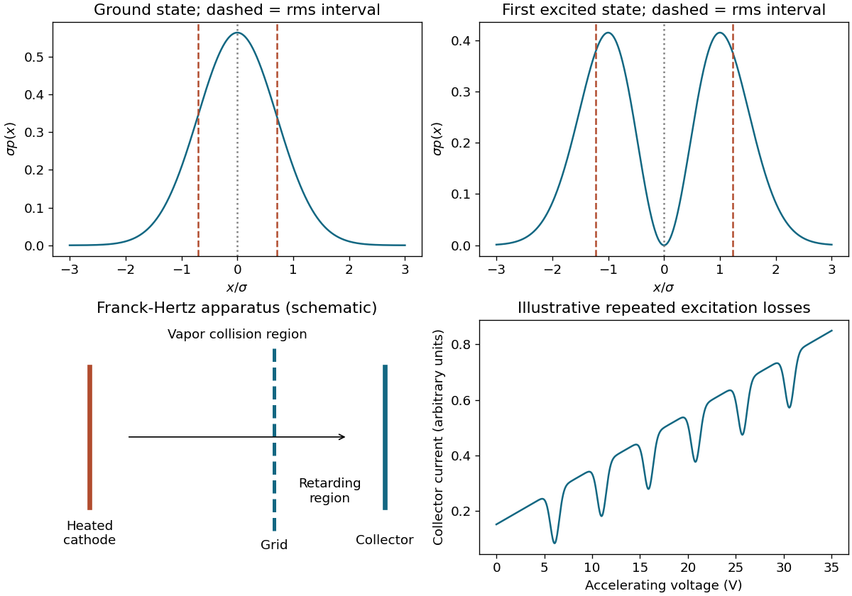
Ground and first-excited oscillator distributions, and an original Franck-Hertz apparatus and signal schematic
. Details. 
Both probability densities are even, so ⟨x⟩=0. The supplied Gaussian moments give ⟨x2⟩0=σ2/2 and ⟨x2⟩1=3σ2/2. Therefore Δx0=σ/2,Δx1=3/2σ. The original plots mark these two symmetric rms intervals around the common mean.
Time evolution gives e−iE0t/ℏ[ϕ0+e−iωtϕ1]/2. It becomes the opposite relative-sign superposition when e−iωt=−1, first at tmin=π/ω. The overlap with the initial state is proportional to 1+e−iωt and vanishes then; global phase is immaterial.
Ancestors (10)
- S3
- 2016
- Past exam of the short options paper shared by Prelims and Parts A and B of the physics course of the University of Oxford
- Short options paper shared by Prelims and Parts A and B of the physics course of the University of Oxford
- Physics course of the University of Oxford
- Undergraduate course of the University of Oxford
- Course of the University of Oxford
- University of Oxford
- List of universities
- Home
Discussion (0)
New discussionThere are no discussions about this article yet.
Articles by others on the same topic (0)
There are currently no matching articles.