Source paper: www.whatdotheyknow.com/request/physics_past_exam_papers_2015_16/response/973997/attach/3/Cowell%20Attachment.zip?cookie_passthrough=1. The dated cover identifies Trinity Term 2016, 14 June. Unlettered marked requests are numbered in source order; explicit letters are retained. All optional Energy Studies alternatives are addressed. S18 is intentionally excluded from new solutions because complete official answers match that section.
The simple poles occur at z=n−α, n∈Z, since the derivative of the sine there is π(−1)n. ThusThere is also a double pole at zero, not included in that list because 0<α<1. Its residue, needed for the next contour calculation, is the derivative of cscπ(z+α) at zero, namely −πcsc(πα)cot(πα).
Resn−αf=π(n−α)2(−1)n.
On the square, ∣z∣≥N. The identity ∣sinπ(x+α+iy)∣2=sin2π(x+α)+sinh2πy bounds the sine away from zero on the vertical sides because x=±N; on horizontal sides it grows exponentially. Therefore the whole contour integral is O(N−1) or smaller and vanishes. The residue theorem then giveswhich proves n∈Z∑(−1)n/(n−α)2=π2cscπαcotπα. Absolute convergence justifies the limiting residue sum.
0=2πi[−πcscπαcotπα+∑n∈Zπ(n−α)2(−1)n],
Separate the n=0 term and pair n with −n. For small α,Compare the constant and quadratic coefficients with the supplied expansion after subtracting α−2. It follows thatThe paired expansion is uniformly summable on any sufficiently small closed interval of α, so coefficient comparison is legitimate.
(n−α)2(−1)n+(n+α)2(−1)n=n22(−1)n+n46α2(−1)n+O(α4/n6).
n≥1∑n2(−1)n=−12π2,n≥1∑n4(−1)n=−7207π4.
A conformal map preserves local oriented angles and has a nonzero local scale factor. For an orientation-preserving complex map this is equivalent to holomorphy with f′(z)=0 at the point concerned. Infinitesimal figures are rotated and uniformly scaled there, but finite shapes need not be preserved: derivative magnitude and direction can vary across a region. Antiholomorphic maps preserve unoriented angles while reversing orientation; the convention being used must be stated.
For real x=−1, w=1−2/(x+1) is real. Its finite image is the entire real axis except w=1, which is approached only as x→±∞. The point x=−1 maps to infinity. On the extended complex plane the extended real axis maps onto itself, with z=∞ mapping to one.
The identity w−1=−2/(z+1) gives ∣w−1∣=2/r on ∣z+1∣=r. Thus the image circle has center one and radius 2/r. Points strictly inside the original circle satisfy ∣w−1∣>2/r; the center itself maps to infinity. The interior therefore becomes the exterior together with infinity on the Riemann sphere, rather than the interior of the image circle. This inversion is a useful warning against assuming conformality preserves global inside/outside assignments.
For z=eiθ, w=itan(θ/2), which is purely imaginary; z=−1 supplies the point at infinity. Conversely, the inverse map is z=(1+w)/(1−w). Requiring ∣w∣=1 is equivalent to ∣z−1∣=∣z+1∣, hence Rez=0, including the appropriate infinite point in the extended-plane formulation. The unit circle and imaginary axis are exchanged, but the real axis is not.
Set z=eiθ. The integral becomesThe roots are z=(−3±2)/(2−i), only z+=−1/(2−i) lying inside. The derivative of the quadratic at z+ is two, so the residue is 1/(2i). Consequently ∫02πdθ/(3+2cosθ+sinθ)=π. The denominator is positive since 3>5, so no principal-value qualification is required.
∮∣z∣=1i[(1−i/2)z2+3z+(1+i/2)]dz.
Cauchy's theorem says that a holomorphic function integrates to zero around a closed contour homologous to zero in its domain. Thus deforming one contour into another without crossing a singularity preserves the integral. More generally for a meromorphic f, the exact condition isEqual winding numbers about every singularity are sufficient. They are not necessary for one particular function because residues can cancel; even arbitrary contours have equal integrals for f=0. A topological deformation criterion must not be confused with a necessary condition for accidental equality.
a∑[nΓ(a)−nΓ′(a)]Resaf=0.
The finite singularities are square-root branch points at z=±1. Choose the cut between them and the branch f(z)∼z at infinity. The two banks then have values +i1−x2 above and −i1−x2 below. A counterclockwise loop around the cut traverses its upper bank right-to-left, so its integral is −2iI, where I is the required real integral. At large radius,Therefore I=π/2. Infinity is not another square-root branch point: this branch has an ordinary pole there on its sheet. Small detours about the finite endpoints vanish as their radius to power 3/2.
f(z)=z−2z1+O(z−3),∮f(z)dz=−πi.
The first law gives elliptical relative orbits with the center of force at a focus; the second gives equal swept areas in equal times, expressing angular-momentum conservation. For circular binary motion, let r1+r2=a and M1r1=M2r2. The force equation M1(2π/P)2r1=GM1M2/a2 givesThe corresponding relation for ellipses uses the relative semimajor axis rather than instantaneous separation.
P2a3=4π2G(M1+M2).
Eclipses justify an approximately edge-on orbit, and equal velocity amplitudes imply equal masses. The relative speed is 200 km s−1, so a=(v1+v2)P/(2π)≃1.50×1010 m, or a≃0.100 AU. Substitution in the binary period law gives M1+M2≃4.52M⊙, hence M1=M2≃2.26M⊙. Inclination corrections scale the dynamical masses as sin−3i if exact edge-on viewing is relaxed.
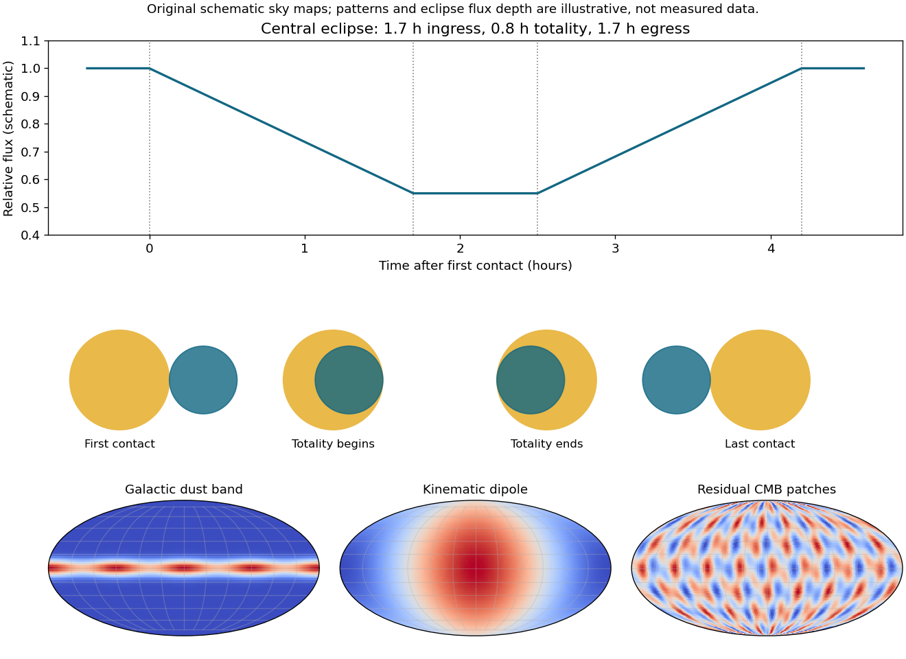
Assume a central eclipse and nearly uniform projected speed during it. Let r be the smaller radius and R the larger. First-to-second contact requires travel 2r, whereas the totality interval requires 2(R−r). With relative speed 200 km s−1,The light curve has ingress, flat minimum and egress lasting 1.7, 0.8 and 1.7 hours. At the four contacts the projected center separations are R+r,R−r,R−r,R+r. A noncentral chord would require an impact parameter and changes the inferred radii; the data alone do not fix that geometry exactly. For comparable masses in an ordinary coeval system, a component larger than its main sequence companion suggests expansion away from the main sequence, conventionally toward a subgiant/early giant track. That is a conditional evolutionary interpretation: neither effective temperature nor a bolometric flux is supplied, so a unique position on the Hertzsprung-Russell diagram cannot be inferred from these radii alone. Binary interactions and the assumed central chord also matter; these numbers do not establish an ordinary single-star evolutionary model.
r=2v(1.7 h)≃6.12×10⁵ km,R=r+2v(0.8 h)≃9.00×10⁵ km.

Hydrostatic balance is dP/dr=−GM(r)ρ/r2. A free-fall estimate gives tdyn∼R⊙3/(GM⊙)≃1.6×103 s; a test particle falling in a fixed point-mass field adds factor π/(22), giving about 30 minutes.
For an ideal nonrelativistic gas with negligible boundary pressure, the virial theorem is 2U+Ω=0, so total energy is Ω/2. Since Ω=−∫0MGmdm/r(m) and r≤R, ∣Ω∣≥GM2/(2R). This is a minimum magnitude, not a lower bound on the negative energy: unrestricted central concentration can make the latter arbitrarily negative. A uniform-density estimate gives Ω=−3GM2/(5R) and available contraction energy 3GM2/(10R). Its release at present solar luminosity lasts t∼107 yr (order 107–108 years for alternative structural estimates), much less than a nuclear-burning lifetime.
Using the supplied atomic masses consistently includes the net electron bookkeeping after positron annihilation. The released fraction is η=(4mH−mHe)/(4mH)≃0.0071, corresponding to about 26.7 MeV per helium nucleus. If 10% of the solar mass is processed and luminosity stays constant, t≃0.1ηM⊙c2/L⊙≃1010 years.
At separation one femtometre the proton Coulomb energy is 1.44 MeV. At 2×10⁷ K, mean thermal kinetic energy 3kBT/2≃2.59 keV, making their ratio about 5.6×10². Classical over-barrier collisions are therefore extremely improbable. Quantum tunnelling through the Coulomb barrier and the high-energy distribution tail allow fusion, with the slow weak-interaction step regulating the proton-proton chain. The reaction summary is a net energy/matter balance, not one simultaneous four-proton collision.
Galactic dust emission is concentrated in a bright band along the Galactic plane, with clumps associated with dust-rich regions. It is a foreground with a spectrum different from a 2.7 K blackbody, so multi-frequency observations can help separate it from the CMB. The schematic below illustrates its geometry rather than reproducing observed sky data.
Motion relative to an isotropic radiation field produces a dipole: one broad hot hemisphere and an opposite cool hemisphere. To first order T(θ)=T0[1+(v/c)cosθ], where θ=0 is the forward direction. This is not a narrow Galactic-plane feature and is not the intrinsic small-scale CMB pattern.
After foreground and dipole removal, primordial CMB anisotropies are small hot and cold patches across the sky, with characteristic correlated angular scales and amplitudes of order 10−5 of the mean temperature. They trace perturbations at photon decoupling and subsequent propagation, not simply the current distribution of Milky Way dust.
Expansion redshifts photon energies and preserves a blackbody spectrum, so a comoving observer at z=2 sees T=T0(1+z)≃8.18 K. A one-sided dipole excess of 0.105% means v/c=0.00105, hence v≃315 kms−1. Motion is toward the hotter region. The peak-to-peak contrast is twice this, so using 0.210% for v/c would double the inferred speed incorrectly.
The given calibration yields MV=−3.5log1050≃−5.946. The distance modulus is 31.446, giving d≃19.5 Mpc if extinction is negligible. Hubble's law predicts vH≃1400 km s−1, compared with 1150 km s−1 observed. The approximately −250 km s−1 difference can be a line-of-sight peculiar velocity of the cluster and observer, together with distance-calibration uncertainties. The local flow need not follow a perfectly smooth expansion law.
Blackbody radiation defeated classical equipartition because it predicts excessive short-wavelength emission. Quantized oscillator energy exchange hν, and ultimately the photon occupation law, gives the Planck spectrum. In the photoelectric effect, electron energy follows light frequency with a threshold, rather than simply increasing with beam intensity; individual photons supply hν and the maximum kinetic energy is hν−W. Intensity chiefly changes the event rate at a fixed frequency. These explain two distinct failures of a purely continuous classical wave-plus-matter model, while retaining wave propagation and interference.
Approximate helium mass by 2mp+2mn≃6.69×10⁻²⁷ kg. Nonrelativistic momentum is p=2mT, giving λ=h/p≃0.203 nm. A transverse width of one micrometre implies a characteristic position uncertainty of that order and a minimum momentum uncertainty of order ℏ/a∼10−28 kg m s−1, with factors depending on profile convention. For a uniform interval Δx=a/12, but an exactly abrupt rectangular wavefunction actually has infinite rms momentum spread. Width alone does not uniquely specify both rms uncertainties; a smooth near-minimum-uncertainty beam is needed for a finite order-of-magnitude estimate.
Immediately after a uniformly illuminated hard slit, the normalized transmitted state is ψ(x)=w−1/2 for ∣x∣<w/2, zero elsewhere. With Fourier convention ψ(p)=(2πℏ)−1/2∫e−ipx/ℏψ(x)dx,The supplied sinc integral verifies unit normalization. The first zeros occur at ±δpx, but this finite central-lobe width is not the rms uncertainty: px2p fails to have a convergent integral.
ψ(px)=2πℏwsinc2ℏpxw,p(px)=δpx1sinc2δpxπpx,δpx=wh.
For an aligned narrower slit placed immediately after the first, uniform illumination gives transmission probability d/w. Conditional on passage the same normalized formula applies with w replaced by d and central-lobe momentum scale h/d. Position rms is d/12, while the exact hard-edge rms Δpx is infinite. Thus the source's finite “uncertainty” can only mean a characteristic diffraction width; the rigorous Heisenberg inequality is not violated, and smoothing the edges restores finite rms moments satisfying it.
A 10 keV X-ray has λ≃0.124 nm. The ideal position-filter probability and momentum formula at fixed aperture widths are unchanged, since the Fourier transform involves h and the aperture geometry. Its larger total momentum makes the angular diffraction width smaller, approximately λ/d. Real slit-material transmission and absorption are additional experimental issues.
To distinguish 2b equal transverse bins across width w, d=w/2b. Six bits gives one-nanometre pixels; ten gives 0.0625 nm, below the helium wavelength. In the stipulated fixed-energy freely propagating beam, the latter entails transverse diffraction momenta comparable to or exceeding the available total momentum and lies outside the paraxial aperture model. Six-bit localization is less demanding, although fine detector resolution and losses remain practical constraints. This is not a universal theorem that an atom can carry at most six bits in every encoding: accessible modes, energy, aperture, measurements and success probabilities define the channel.
The equation is iℏ∂tψ=[−ℏ2∂x2/(2m)+V(x)]ψ. The generator of time evolution is the sum of kinetic and potential energy operators. For a sharp stationary energy, insert ψ(x,t)=ϕ(x)e−iEt/ℏ to obtain [−ℏ2ϕ′′/(2m)+Vϕ]=Eϕ. The probability in dx is ∣ψ∣2dx, normalized to one; hence a normalized one-dimensional wavefunction has dimensions length−1/2. Its overall phase is unobservable, but relative phase affects interference.
Integrating F=−kx gives V=kx2/2 up to a constant. Thus −ℏ2ϕ′′/(2m)+mω2x2ϕ/2=Eϕ, with ω=k/m. The potential is a symmetric upward parabola and tends to infinity in both directions; normalizable states decay at large ∣x∣.
For the Gaussian, ϕ0′′=(x2/σ4−1/σ2)ϕ0. Using ℏ/(mω)=σ2, the x2 terms cancel and leave E0=ℏω/2. For ϕ1∝xϕ0, differentiation gives ϕ1′′=(x2/σ4−3/σ2)ϕ1, and the same cancellation gives E1=3ℏω/2. The normalization constants do not affect these eigenvalue equations.
Squaring the states gives p0=e−x2/σ2/(πσ),p1=2x2e−x2/σ2/(πσ3). The first peaks at zero; the second has a node there and peaks at x=±σ. For a centered interval of width δx≪σ, P0≃δx/(πσ), whereas P1≃(δx)3/(6πσ3). Its leading linear term vanishes, but the probability in a finite interval is not exactly zero.
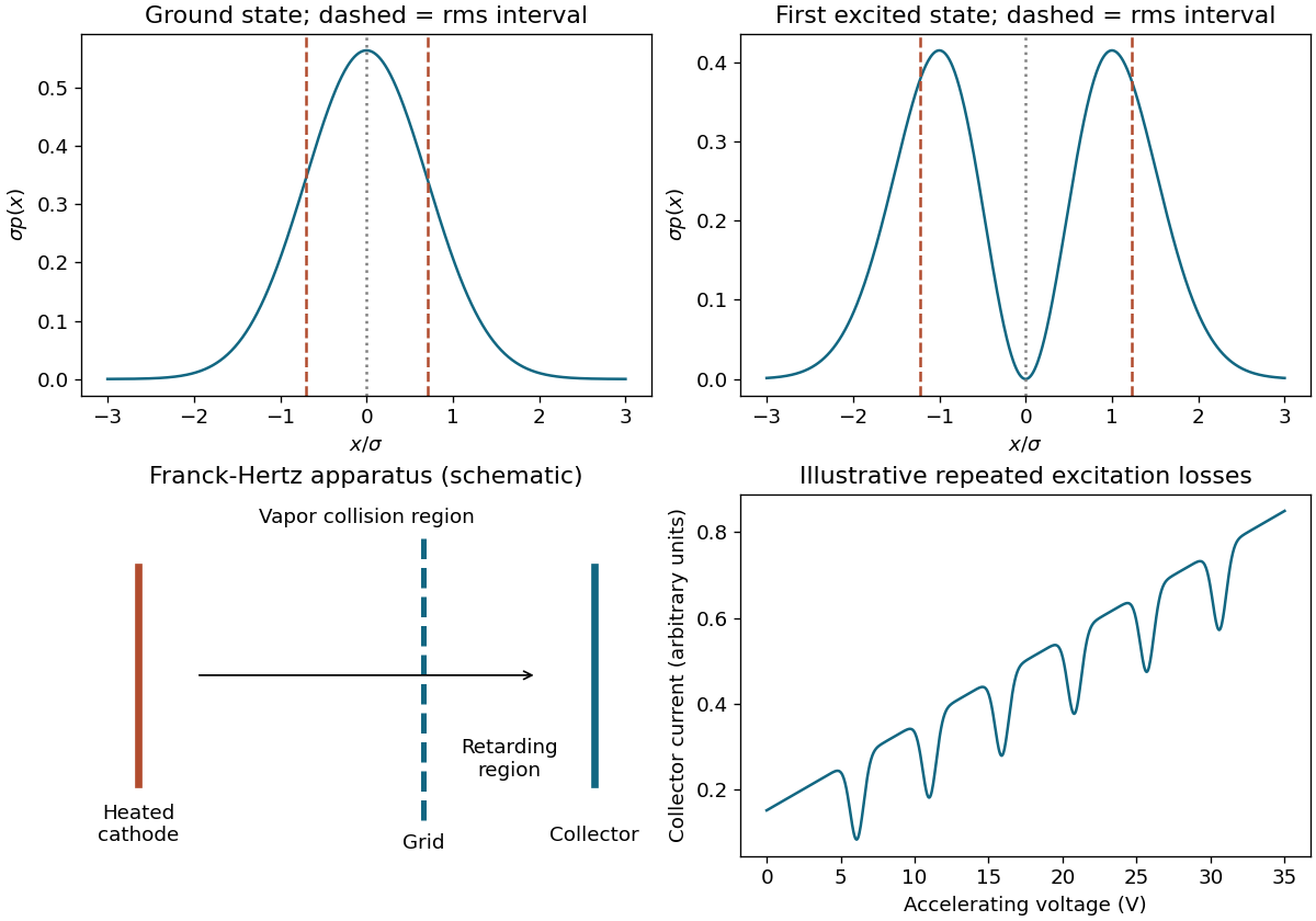
Ground and first-excited oscillator distributions, and an original Franck-Hertz apparatus and signal schematic
. Details. 
Both probability densities are even, so ⟨x⟩=0. The supplied Gaussian moments give ⟨x2⟩0=σ2/2 and ⟨x2⟩1=3σ2/2. Therefore Δx0=σ/2,Δx1=3/2σ. The original plots mark these two symmetric rms intervals around the common mean.
Time evolution gives e−iE0t/ℏ[ϕ0+e−iωtϕ1]/2. It becomes the opposite relative-sign superposition when e−iωt=−1, first at tmin=π/ω. The overlap with the initial state is proportional to 1+e−iωt and vanishes then; global phase is immaterial.
A heated cathode emits electrons into low-pressure atomic vapor, and a variable accelerating voltage gives them kinetic energy. A grid and small retarding region precede the collecting anode. Below the first excitation threshold most collisions are elastic; above it, electrons can transfer a definite excitation energy to atoms and may then fail to overcome the collector's retarding field. Collector current develops repeated minima as accelerating voltage increases, separated by roughly the same excitation voltage, approximately 4.9 V for mercury. Contact potentials and energy spreads shift or smear the minima without removing their characteristic spacing. A smooth loss mechanism would not produce these repeated fixed-energy thresholds.[ref]
A classically accelerating Coulomb electron radiates and loses orbital energy, so a stable nonradiating orbit is impossible within that unmodified theory. Bohr instead postulates stationary nonradiating orbits, quantized angular momentum μvr=nℏ and photon emission/absorption with hν=Ei−Ef. Here μ=meM/(me+M) describes relative motion. The angular-momentum condition is the standing-wave relation 2πr=nλdB for the relative orbit. These are additional quantum postulates, not consequences of classical radiation theory.
Coulomb centripetal balance and μvr=nℏ giveThe radius is the electron-nucleus separation. For positronium, Z=1 and μ=me/2, so rn=2a0n2 and En=−Ry/(2n2). Each constituent's radius about the center of mass is half the separation; calling both that radius and rn the orbital radius without distinction would create another factor-two error.
rn=μmeZa0n2,En=−meμn2Z2Ry.
The relative orbital speed is Ze2/(4πϵ0ℏn). Divide the circumference by this speed to findPositronium has twice the hydrogen period at the same principal quantum number. The symbol n here labels principal levels with n=1 the ground state; if “nth excited state” is read literally as excitation count, replace n by n+1.
Tn=Z2μe44ϵ02h3n3.
The Lyman-alpha gap is 3Z2(μ/me)Ry/4, giving λ=4hc/[3Z2(μ/me)Ry]. For heavy lithium nucleus and Z=3, λ≃13.5 nm. A specified lithium isotope would permit the small reduced-mass correction; no isotope is supplied.
Positronium has Z=1 and half the hydrogen reduced-mass energy scale, so λ≃243 nm. The large contrast with lithium is mainly Z2 Coulomb scaling, with an additional factor two from the moving positron's equal mass. It is not explained by a different photon propagation law.
A tokamak confines a hot, approximately toroidal plasma using a strong toroidal magnetic field and a poloidal field associated with plasma current and external coils. Helical field lines and suitable magnetic surfaces reduce rapid transverse escape. D-T fusion releases 17.6 MeV, mostly in an uncharged neutron that escapes magnetic confinement and transfers energy to a surrounding blanket. A heat exchanger and thermal power cycle convert some of that energy into electricity.
Essential systems include the vacuum vessel, toroidal and poloidal magnets, current-drive/transformer and auxiliary heating equipment, fueling and exhaust systems, divertor for concentrated heat and particle removal, neutron-absorbing/breeding blanket and shielding. Alpha particles retained in the plasma contribute self-heating. Confinement and controlled exhaust are as important as reaching a high temperature; a magnetic field does not confine the neutrons or make material heat loads vanish.
Lithium in the blanket breeds tritium through neutron reactions, notably 6Li+n→4He+T. Tritium is not abundant enough in nature to supply a large reactor fleet without breeding. The blanket must also transfer heat and manage neutron damage and losses, and the breeding ratio must exceed consumption after accounting for processing and inventory. Lithium is therefore a fuel-cycle resource rather than the primary charged plasma reactant in the D-T core.
Extraction energy is 6000 kg×2500 kWhkg−1=15 GWh per year. A continuously operating 2 GW electrical plant generates 17.5 TWh per year, so lithium extraction consumes about 0.086% of its output under the stated estimate. This is energetically favorable even before claiming anything about capital costs or extraction feasibility.
For an ocean mass about 1.4×10²¹ kg, concentration 0.17 ppm implies about 2.4×10¹⁴ kg lithium. At the specified consumption/output ratio, a hypothetical 20 TW electric world would use 6×10⁷ kg annually, giving roughly 4×10⁶ years. For 3 TW the corresponding scale is 3×10⁷ years. State the assumed demand: “power the world” does not uniquely specify electric demand versus primary-energy use. These are inventory quotients ignoring growth, accessible fraction, ecological constraints and processing throughput.
Mean kinetic energy 3kBT/2=12.9 keV means T=8.6 keV, not 12.9 keV. For fully ionized D-T with equal electron and ion temperatures, p=2nikBT gives ni≃4.90×10¹⁹ m−3. Thusonly about one third of the stated requirement. The specified operating point therefore does not meet that criterion and requires improved confinement/pressure or continuing external heating. If the criterion's n counts all thermal particles instead of ions, the product doubles but remains below its given threshold. A precise fusion gain or duty cycle cannot be inferred from the triple product alone.
niτET≃1.05×10²¹ m−3skeV,
Articles were limited to the first 100 out of 315 total.
Ancestors (8)
- Past exam of the short options paper shared by Prelims and Parts A and B of the physics course of the University of Oxford
- Short options paper shared by Prelims and Parts A and B of the physics course of the University of Oxford
- Physics course of the University of Oxford
- Undergraduate course of the University of Oxford
- Course of the University of Oxford
- University of Oxford
- List of universities
- Home
Discussion (0)
New discussionThere are no discussions about this article yet.
Articles by others on the same topic (0)
There are currently no matching articles.