At equal sample count, rejection sampling eventually has smaller variance for fixed ; at equal expected proposal cost, importance sampling eventually wins. The distinction matters because a sample of the rejection sampling estimator means an accepted draw.
For the importance sampling estimator, all coordinates contribute to the importance weight although only one enters the integrand. The same normal distribution transform as in (c), now with linear coefficient for coordinate one, givesBoth estimators are unbiased estimators of , andFor fixed , the first variance grows exponentially while the second stays constant. This is the benefit of returning exact target draws in rejection sampling. However, obtaining those draws costs proposals each on average.
To compare computational work, multiply each variance by its expected proposal count. For importance sampling that count is ; for rejection sampling it is . The ratio of the resulting cost-normalized variances isbecause . Thus importance sampling eventually gives better precision for the same expected number of proposals, assuming comparable work per proposal. This is an asymptotic cost comparison, not a guarantee that a fixed small computing budget produces any accepted draws. Both methods still deteriorate exponentially in this comparison. For they coincide and every proposal is accepted.
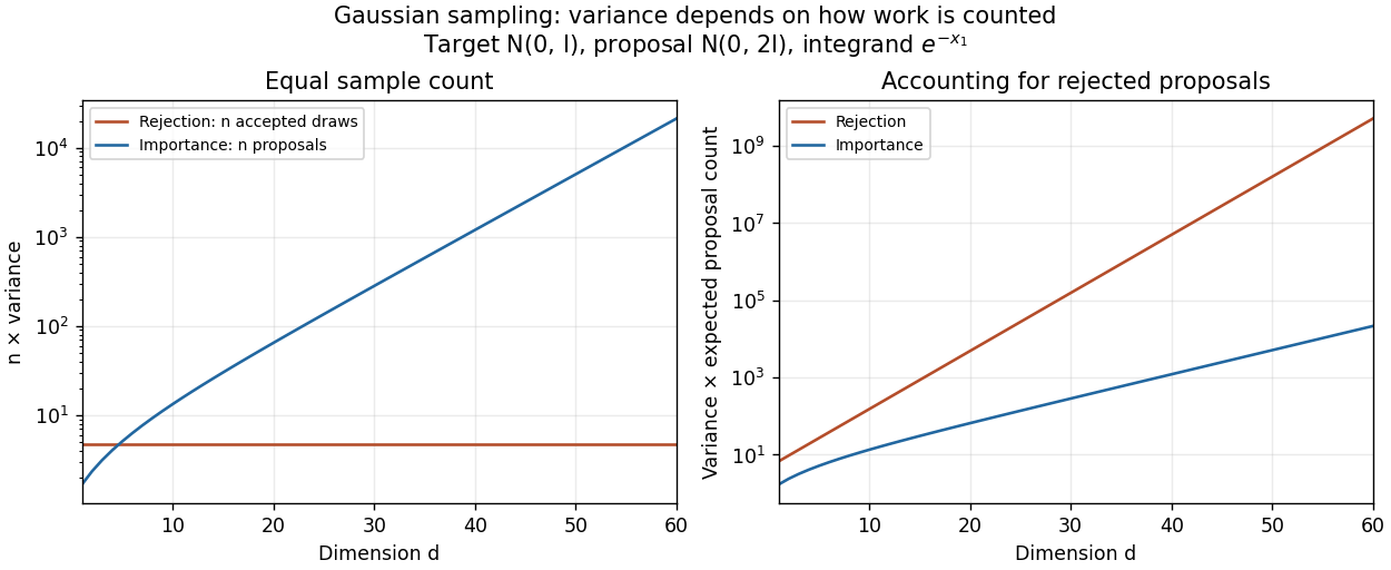
Sample-count and expected-proposal-cost comparisons for the one-coordinate integrand at sigma squared equal to two
. Details. 
A practical improvement is to exploit the integrand's one-coordinate structure directly: average for standard normal distribution draws , without generating unused coordinates. The optimal change of proposal distribution in (iii) improves further.
Articles by others on the same topic
There are currently no matching articles.