Simulation and statistical programming course of the University of Oxford (A12)

a

i

Solution

Generate independent and identically distributed random variables

X_{1}, \dots, X_{n}

with probability density function

p

, evaluate

ϕ (X_{i})

for each draw, and return the Monte Carlo estimator

θ_{n}^{MC} = \frac{1}{n} i = 1 \sum n ϕ (X_{i}) .

Linearity of expectation makes this an unbiased estimator:

E θ_{n}^{MC} = θ

. Independence and the specified variance give

Var (θ_{n}^{MC}) = 1/ n

. Its Monte Carlo standard error is therefore

n^{- 1/2}

, and the strong law of large numbers gives convergence to

θ

almost surely.

ii

Solution

Apply Chebyshev's inequality to the Monte Carlo estimator:

P (θ_{n}^{MC} - θ \geq 0.01) \leq \frac{Var ( θ _{n}^{MC} )}{0.0 1 ^{2}} = \frac{1 0 ^{4}}{n} .

Thus

1 0^{4} / n \leq 0.01

suffices, giving

n = 1, 000, 000.

This is a finite-sample probability guarantee for every target satisfying the given variance assumption. It is a sufficient sample count supplied by the inequality, rather than a claim that every such target actually needs a million draws.

iii

Solution

The central limit theorem gives

n (θ_{n}^{MC} - θ) \Rightarrow N (0, 1)

, so, with

Φ

the cumulative distribution function of the standard normal distribution,

P (θ_{n}^{MC} - θ < 0.01) \approx 2Φ (0.01 n) - 1.

The error has two tails. Using the supplied

2.58

quantile, whose two-sided coverage is approximately

0.9902

, gives

0.01 n \geq 2.58, N := n = ⌈ \frac{2.5 8 ^{2}}{0.0 1 ^{2}} ⌉ = 66, 564.

The supplied

2.33

quantile would be appropriate for a one-sided

99%

calculation; it would give only approximately

98.02%

two-sided coverage. Using the exact

0.995

quantile instead of

2.58

would give

66, 349

draws; we consistently use the paper's rounded value

N = 66, 564

below.

For routine Monte Carlo integration, the central limit theorem calculation is preferable as a practical budget: it uses about one fifteenth as many draws as the Chebyshev's inequality bound. However, its coverage is approximate. Finite variance alone supplies no universal rate of convergence to the normal distribution; an integrand with large skewness or a heavy-tailed distribution can make the approximation poor even at a large sample count. If an unconditional finite-sample

99%

guarantee is required under only the stated assumptions, use the Chebyshev's inequality budget.

b

i

Solution

Integrating the envelope

p \leq Mq

shows

M \geq 1

. One trial of rejection sampling draws

Y \sim q

and an independent

U

from the uniform distribution on

(0, 1)

, and accepts

Y

U \leq p (Y) / (Mq (Y))

. Repeat with fresh independent random variables after each rejection. Ratios need only be evaluated where

q > 0

; the envelope makes the target zero wherever

q = 0

For any measurable set

B

, integration of the conditional probability of acceptance gives

P (Y \in B, accept) = \int_{B} q (y) \frac{p ( y )}{Mq ( y )} d y = \frac{1}{M} \int_{B} p (y) d y .

Taking the whole domain gives acceptance probability

1/ M

, and dividing gives

P (Y \in B ∣ accept) = \int_{B} p (y) d y

. Fresh trials therefore supply independent and identically distributed random variables

X_{1}, \dots, X_{m}

with target probability density function

p

. The corresponding Monte Carlo estimator is

θ_{m}^{RS} = \frac{1}{m} j = 1 \sum m ϕ (X_{j}) .

The proposal count

T

up to and including one acceptance has the geometric distribution

P (T = t) = (1 - 1/ M)^{t - 1} / M, t = 1, 2, \dots, E T = M .

For example, the tail-sum formula gives

E T = \sum_{t \geq 0} (1 - 1/ M)^{t} = M

. Thus the expected cost is

M

proposal draws per accepted target draw.

ii

Solution

Stop rejection sampling when exactly

N = 66, 564

target draws have been accepted. The total proposal count

T_{N}

is a sum of

N

independent waiting times with geometric distribution, equivalently a negative binomial distribution counting trials. Consequently

E T_{N} = MN = 66, 564 M, Var (T_{N}) = NM (M - 1) .

The accepted-sample Monte Carlo estimator then has the approximate

99%

precision from (a)(iii). The displayed proposal cost is an expected value, which need not be an integer. Spending this many proposals in advance does not ensure that

N

target draws will have been accepted.

iii

Solution

With a fixed budget of

n

independent proposal trials, the accepted count

K_{n}

has binomial distribution with success probability

1/ M

. Hence

E K_{n} = \frac{n}{M}, Var (K_{n}) = \frac{n ( M - 1 )}{M ^{2}} .

For

M > 1

, the central limit theorem gives the one-sided approximation

P (K_{n} \geq N) \approx Φ (\frac{n - MN}{n ( M - 1 )}) .

Use

z = 2.33

, since now only the lower tail of the accepted count matters. Requiring

n - MN \geq z n (M - 1)

and solving the resulting quadratic equation in

t = n

gives the one-sided normal approximation for a rejection proposal budget

n_{0} = (\frac{z M - 1 + z ^{2} ( M - 1 ) + 4 MN}{2})^{2} .

Equivalently, before rounding, this is

MN + z^{2} (M - 1) /2 + (z /2) (M - 1) [z^{2} (M - 1) + 4 MN]

. For the value in (a)(iii),

n_{0} = (\frac{2.33 M - 1 + 5.4289 ( M - 1 ) + 266256 M}{2})^{2} .

When

M = 1

, every proposal is accepted and

n_{0} = N = 66, 564

exactly. Otherwise the positive safety margin above

MN

allows for random fluctuations in the number accepted. The average cost in (b)(ii) describes stopping at the

N

th acceptance; this answer chooses a deterministic budget that reaches that acceptance with approximately

99%

probability.

The approximation requires a sufficiently accurate normal distribution approximation to the binomial distribution. An exact

99%

budget can instead be found from its tail probabilities. Also, a

99%

chance of enough accepted draws and approximate

99%

precision conditional on obtaining them are separate claims: their intersection is not automatically a

99%

event.

c

i

Solution

Draw independent and identically distributed random variables

Y_{1}, \dots, Y_{n} \sim q

and use the importance weight

w = p / q

. The importance sampling estimator is

θ_{n}^{IS} = \frac{1}{n} i = 1 \sum n w (Y_{i}) ϕ (Y_{i}) .

The envelope supplies the support condition for importance sampling. Since

E_{q} [w (Y) ϕ (Y)] = E_{p} ϕ (X) = θ

, this is an unbiased estimator. Moreover,

0 \leq w \leq M

, so

E_{q} [w (Y)^{2} ϕ (Y)^{2}] = \int w (x) ϕ (x)^{2} p (x) d x = E_{p} [w (X) ϕ (X)^{2}] \leq M E_{p} [ϕ (X)^{2}] = M (1 + θ^{2}) .

Here

E_{p} ϕ^{2} = Var_{p} (ϕ) + θ^{2} = 1 + θ^{2}

. Subtracting the squared expected value and dividing by

n

proves the bounded-weight importance-sampling moment bound in the requested form:

Var (θ_{n}^{IS}) = \frac{E _{p} [ w ϕ ^{2} ] - θ ^{2}}{n} \leq \frac{M + ( M - 1 ) θ ^{2}}{n} .

ii

Solution

The definition of

a

and (c)(i) give

a \leq M

. Nonnegativity of the variance strengthens the lower bound to

\frac{θ ^{2}}{1 + θ ^{2}} \leq a \leq M .

In fact the variance of one weighted observation is exactly

v_{IS} := Var_{q} (w (Y) ϕ (Y)) = a (1 + θ^{2}) - θ^{2} .

It is finite by the envelope. For

v_{IS} > 0

, the central limit theorem gives approximate two-sided coverage

2Φ (0.01 n / v_{IS}) - 1

, so the paper's rounded quantile yields

n_{IS} = ⌈ 66, 564 [a (1 + θ^{2}) - θ^{2}] ⌉ .

v_{IS} = 0

, the weighted observation equals

θ

almost surely, and one draw is sufficient. These are theoretical budgets:

a

and

θ

may themselves be unknown and need preliminary estimation in an implementation.

Compare with the average rejection sampling cost

66, 564 M

. Ignoring integer rounding, importance sampling uses fewer proposal draws at the same approximate precision precisely when

a (1 + θ^{2}) - θ^{2} < M, a < \frac{M + θ ^{2}}{1 + θ ^{2}} .

For literal integer budgets, the comparison is

⌈ 66, 564 v_{IS} ⌉ < 66, 564 M

. The simpler strict inequality is the intended leading-order condition. The bound

a \leq M

alone does not ensure an improvement when

θ \neq = 0

; this is a proposal-budget variance comparison of importance and rejection sampling.

2

a

i

Solution

Write

w = p / q

where

q > 0

, assigning zero elsewhere. The envelope ensures

0 \leq w / M \leq 1

, and

π

is nonnegative. Integrating its joint probability density over the auxiliary coordinate gives

\int_{0}^{1} π (x, u) d u = Mq (x) \frac{w ( x )}{M} = p (x) .

Consequently

\int_{Ω} \int_{0}^{1} π (x, u) d u d x = \int_{Ω} p (x) d x = 1

. This proves normalization of a probability distribution; the change of integration order is justified by Tonelli's theorem.

The coordinates are generally dependent. For

p (x) > 0

, their conditional probability density is

π (u ∣ x) = \frac{M}{w ( x )} 1_{[0, w (x) / M]} (u) .

Thus

U ∣ X = x

has a uniform distribution on an interval whose endpoint depends on

x

. They are independent exactly when

w (x)

is constant for

p

-almost every

x

, since only then do these conditional laws agree. In particular,

p = q

is an exception:

X \sim p

and

U \sim Unif (0, 1/ M)

are independent. An unconditional answer that they can never be independent would therefore be too strong.

ii

Solution

Integrating the joint probability density over the auxiliary coordinate, as in (i), gives the marginal distribution

π_{X} (x) = \int_{0}^{1} π (x, u) d u = p (x) .

In particular, augmenting with

U

preserves the target probability distribution of

X

. The other marginal distribution, though not needed to identify

X

, is

π_{U} (u) = M \int_{Ω} q (x) 1_{{w (x) \geq M u}} d x

for

0 < u < 1

. It need not be a uniform distribution on

(0, 1)

iii

Solution

For the proposed joint probability density

ρ

, define the acceptance indicator function

A_{i} := 1_{{V_{i} \leq w (Y_{i}) / M}} .

On the proposal's support the importance weight is

π (Y_{i}, V_{i}) / ρ (Y_{i}, V_{i}) = M A_{i}

. Therefore the requested augmented-space importance sampling estimator is

θ_{n}^{IS} = \frac{M}{n} i = 1 \sum n A_{i} ϕ (Y_{i}) .

Its expected value is

θ

, provided

E_{p} ∣ ϕ (X) ∣ < \infty

. This is not the ordinary estimator

n^{- 1} \sum_{i} w (Y_{i}) ϕ (Y_{i})

from question 1. Taking the conditional expectation of this augmented estimator given all

Y_{i}

produces that ordinary estimator, because

E [A_{i} ∣ Y_{i}] = w (Y_{i}) / M

. This is the Rao-Blackwell identity for a fixed-denominator rejection estimator.

iv

Solution

Use the same acceptance indicator functions and set

K_{n} = \sum_{i = 1}^{n} A_{i}

S_{n} = \sum_{i = 1}^{n} A_{i} ϕ (Y_{i})

. The rejection sampling estimator based on these

n

proposals is the mean over the accepted observations:

θ_{n}^{RS} = \frac{S _{n}}{K _{n}} (K_{n} > 0) .

For

K_{n} = 0

, any fixed convention, such as zero, is harmless asymptotically. The

A_{i}

are independent and identically distributed random variables with Bernoulli distribution and success probability

1/ M

, so the strong law of large numbers gives

K_{n} / n \to 1/ M

almost surely. In particular

K_{n} > 0

eventually almost surely. The exact identity

θ_{n}^{IS} = \frac{M K _{n}}{n} θ_{n}^{RS}

then holds whenever

K_{n} > 0

. Wherever

S_{n} \neq = 0

, it follows that

\frac{θ _{n}^{IS}}{θ _{n}^{RS}} = \frac{M K _{n}}{n} ⟶ 1 almost surely .

A qualification is missing from the printed claim: the quotient must be defined eventually. A convenient sufficient assumption is

E_{p} ∣ ϕ ∣ < \infty

and

θ \neq = 0

. Indeed, another application of the strong law of large numbers gives

S_{n} / n \to θ / M

, ensuring that

S_{n}

is eventually nonzero. This proves the stated quotient limit under that assumption.

As printed, the assertion is false as a universally defined quotient. For example,

ϕ \equiv 0

makes both estimates zero for every

n

. Even excluding that example is insufficient: take

p = q

to be the uniform distribution on

(0, 1)

M = 1

, and

ϕ (y) = 1

for

y < 1/2

and

- 1

otherwise. Then

S_{n}

is a simple symmetric random walk, which returns to zero infinitely often almost surely, leaving the quotient undefined infinitely often.

With integrability but no assumption

θ \neq = 0

, the exact multiplicative identity remains valid, and both estimates converge to

θ

almost surely. In particular

θ_{n}^{IS} - θ_{n}^{RS} \to 0

almost surely. One may alternatively define the quotient's removable

0/0

cases as

M K_{n} / n

; that explicitly extended quantity always converges to one. These are valid repairs of the source's unrestricted statement.

b

i

Solution

Fix a proposal

y

with

q (y) > 0

, and abbreviate

B = M q (y)

H = h (y)

and

P = p (y)

. The envelope says

0 \leq H \leq P \leq B

. Assuming fresh independent uniform distribution draws at both stages, the law of total probability gives

P (accept ∣ Y = y) = \frac{H}{B} + (1 - \frac{H}{B}) \frac{P - H}{B - H} = \frac{H}{B} + \frac{P - H}{B} = \frac{p ( y )}{M q ( y )} .

The second term includes both reaching the residual test and passing it. If

H = B

, the envelope forces

P = B

and the first test accepts with probability one; the second-stage

0/0

ratio is never evaluated. This is squeeze rejection sampling.

ii

Solution

Average the conditional probability in (i) over

Y \sim q = q / Z_{q}

P (accept) = \int_{Ω} \frac{q ( y )}{Z _{q}} \frac{p ( y )}{M q ( y )} d y = \frac{1}{M Z _{q}} \int_{Ω} p (y) d y = \frac{Z _{p}}{M Z _{q}} .

This is exactly the acceptance mass for an unnormalized rejection envelope. In normalized form the envelope is

p \leq (M Z_{q} / Z_{p}) q

, giving the same acceptance probability. Here

M

bounds the ratio of the unnormalized functions, so its value need not equal the envelope constant for the normalized probability density functions.

The squeeze changes the number of expensive target evaluations, while preserving the per-proposal acceptance probability. The expected number of proposals per accepted draw is

M Z_{q} / Z_{p}

iii

Solution

For a measurable set

C

, (i) gives the joint acceptance probability

P (Y \in C, accept) = \int_{C} \frac{q ( y )}{Z _{q}} \frac{p ( y )}{M q ( y )} d y = \frac{1}{M Z _{q}} \int_{C} p (y) d y .

Divide by

Z_{p} / (M Z_{q})

from (ii). The resulting conditional probability is

P (Y \in C ∣ accept) = \frac{1}{Z _{p}} \int_{C} p (y) d y = \int_{C} p (y) d y .

Thus every accepted value has target probability density function

p

. Repeating rejected trials with fresh independent random variables does not change this law: the contribution from acceptance on trial

j

is multiplied by

(1 - Z_{p} / (M Z_{q}))^{j - 1}

, and summing that geometric series gives the same conditional law. Independent repetitions produce independent target draws.

iv

Solution

The proposal's normalization of a probability distribution is

Z_{q} = \int_{R} e^{- ∣ x ∣} d x = 2, q (x) = \frac{1}{2} e^{- ∣ x ∣} .

This is the Laplace distribution with location zero and scale one. For example, generate its magnitude from the exponential distribution with rate one and give it an independent fair sign. The target is the standard normal distribution, with

Z_{p} = 2 π

To obtain the tight envelope, let

t = ∣ x ∣

. By completing the square,

\frac{p ( x )}{q ( x )} = e^{- t^{2} /2 + t} = e^{1/2} e^{- (t - 1)^{2} /2} \leq e^{1/2} .

Equality occurs at

x = \pm 1

, so

M_{*} = e

is the smallest valid envelope constant. It maximizes the acceptance probability for this fixed proposal. The supplied lower bound must be clipped at zero to satisfy the algorithm's nonnegativity requirement:

h (x) = max {0, 1 - x^{2} /2} .

This is valid because

e^{- s} \geq 1 - s

for

s \geq 0

, while

p

is everywhere positive. Its support is

[- 2, 2]

Here is the fully specified squeeze rejection sampling procedure. Draw

Y

with probability density function

q (y) = e^{- ∣ y ∣} /2

, independently draw

U \sim Unif (0, 1)

, and compute

H = max (0, 1 - Y^{2} /2)

and

B = e e^{- ∣ Y ∣}

. If

U \leq H / B

, return

Y

immediately. Otherwise evaluate

P = e^{- Y^{2} /2}

, independently draw

V \sim Unif (0, 1)

, and return

Y

V \leq (P - H) / (B - H)

. On rejection restart with fresh draws. In this example

B > H

everywhere, so the residual denominator is positive.

Avoiding a target evaluation means accepting at the first test. Its unconditional probability for one proposal is

P (no target evaluation) = \int_{R} q (y) \frac{h ( y )}{M q ( y )} d y = \frac{1}{2 e} \int_{- 2}^{2} (1 - y^{2} /2) d y = \frac{2 2}{3 e} \approx 0.571843.

For comparison, the overall acceptance probability is

2 π / (2 e) = π / (2 e) \approx 0.760173

. The first-stage saving

0.571843

is the fraction of proposals requiring no target evaluation, including both eventual accepted and rejected proposals in the denominator; it is not conditional on acceptance.

3

a

Solution

The following R code implements the given recursion for the Cholesky decomposition. The input is assumed to be a real symmetric matrix that is a positive-definite matrix.

mychol <- function(A) {
  n <- nrow(A)
  if (n == 1L) return(matrix(sqrt(A[1L, 1L]), 1L, 1L))
  j <- 2L:n
  L <- matrix(0, n, n)
  L[1L, 1L] <- sqrt(A[1L, 1L])
  b <- A[j, 1L, drop = FALSE] / L[1L, 1L]
  L[j, 1L] <- b
  S <- A[j, j, drop = FALSE] - tcrossprod(b)
  L[j, j] <- mychol(S)
  L
}

Here tcrossprod(b) is the outer product

b b^{T}

. The drop = FALSE arguments preserve matrix dimensions, including the final one-by-one subproblem, and the base case also returns a matrix.

To verify correctness, partition

A = (a r r^{T} B)

. The code sets

ℓ = a

b = r / ℓ

and recursively factors

S = B - b b^{T}

. This Schur complement is a positive-definite matrix: for

z \neq = 0

z^{T} S z = (- r^{T} z / a z)^{T} A (- r^{T} z / a z) > 0.

C C^{T} = S

is the recursive answer, then the returned lower triangular matrix satisfies

L = (ℓ b 0 C), L L^{T} = (a ℓ b ℓ b^{T} b b^{T} + C C^{T}) = (a r r^{T} B) = A .

The one-dimensional identity starts this mathematical induction proof. Each recursive call reduces the matrix size by one and therefore terminates.

b

Solution

An inverse matrix exists only if the lower triangular matrix has no zero diagonal entries; this necessary assumption is implicit in the request for

L^{- 1}

. Partition

L = (a b 0 C) .

Writing its inverse in the same block form and multiplying gives the recursive inverse of a lower triangular matrix:

L^{- 1} = (a^{- 1} - C^{- 1} b / a 0 C^{- 1}) .

Indeed the lower-left block of the product is

b / a - C (C^{- 1} b / a) = 0

, and the diagonal blocks are identities. This gives an implementation with no call to solve:

ltinv <- function(L) {
  n <- nrow(L)
  if (n == 1L) return(matrix(1 / L[1L, 1L], 1L, 1L))
  j <- 2L:n
  Cinv <- ltinv(L[j, j, drop = FALSE])
  B <- matrix(0, n, n)
  B[1L, 1L] <- 1 / L[1L, 1L]
  B[j, j] <- Cinv
  B[j, 1L] <- -as.vector(Cinv %*% L[j, 1L, drop = FALSE]) / L[1L, 1L]
  B
}

The preserved matrix dimensions also handle

n = 2

. A mathematical induction using the block identity proves that every returned matrix is the desired inverse. Applied to the Cholesky decomposition from (a), all diagonal entries are positive, so all divisions are valid.

c

i

Solution

Each state has exactly

k (n - k)

neighbours: choose one occupied coordinate and one unoccupied coordinate to swap. The normalized proposal distribution is therefore

q (v ∣ u) = \frac{1}{k ( n - k )} 1_{{v \sim u}} .

The swap relation is symmetric and the number of neighbours is constant, so

q (v ∣ u) = q (u ∣ v)

. The discrete uniform distribution used as the prior distribution is also constant on

S_{k}

, with mass

(k n)^{- 1}

. Both factors cancel in the Metropolis–Hastings acceptance probability.

Let

Q = Σ^{- 1}

and

d = v - u

. The displayed multivariate normal distribution presupposes that the covariance matrix

Σ

is a positive-definite matrix, so

Q

is a symmetric matrix. Expanding the difference of quadratic forms gives

lo g \frac{π ( v ∣ x )}{π ( u ∣ x )} = - \frac{1}{2} {(x - v)^{T} Q (x - v) - (x - u)^{T} Q (x - u)} = d^{T} Q (x - u) - \frac{1}{2} d^{T} Q d = d^{T} Q (x - \frac{u + v}{2}) .

Consequently

lo g α (u, v) = min {0, (v - u)^{T} Σ^{- 1} (x - \frac{u + v}{2})} .

The truncation at zero is essential: a log acceptance ratio can be positive, but the logarithm of an acceptance probability cannot.

For the particular proposed swap, let

a = i_{1}

be the coordinate changing from zero to one and

b = i_{2}

the coordinate changing from one to zero. Then

d = e_{a} - e_{b}

, and the untruncated scalar simplifies further to

(Q (x - u))_{a} - (Q (x - u))_{b} - \frac{1}{2} (Q_{aa} + Q_{bb} - 2 Q_{ab}) .

Only two rows and four entries of

Q

are needed for this evaluation. This is Metropolis sampling on fixed-cardinality subsets.

ii

Solution

The source's function name suggests a log return value, and (c)(i) asks for

lo g α

, while the wording here and in (c)(iv) asks for the acceptance probability. We use the literal probability-returning convention and explicitly exponentiate the result of (c)(i):

mylogapp <- function(x, u, v, sigma_inv) {
  d <- v - u
  log_ratio <- as.numeric(crossprod(d, sigma_inv %*% (x - (u + v) / 2)))
  log_alpha <- min(0, log_ratio)
  exp(log_alpha)
}

Thus mylogapp returns

α \in [0, 1]

, and (c)(iv) compares it directly with a uniform distribution draw. Taking the minimum before exponentiating prevents overflow. The arguments

u, v

are assumed to be valid neighbouring states. A log-returning convention would instead return log_alpha and compare log(runif(1)) with it; the two conventions implement the same Metropolis–Hastings algorithm, provided the caller uses the matching comparison.

iii

Solution

The Cholesky decomposition gives

Σ = L L^{T}

. If

B = L^{- 1}

, reversal of factors in a matrix inverse gives

Σ^{- 1} = (L^{T})^{- 1} L^{- 1} = B^{T} B .

Hence the required R implementation is

invsigma <- function(sigma) {
  L <- mychol(sigma)
  B <- ltinv(L)
  crossprod(B)
}

Here crossprod(B) computes

B^{T} B

. Using tcrossprod(B) would compute

B B^{T}

, which generally differs from

Σ^{- 1}

. Both helper functions preserve the one-by-one matrix case.

iv

Solution

Choose

k

distinct coordinates uniformly for the starting ones; each element of

S_{k}

then has starting probability

1/ (k n)

. At each iteration choose one current one and one current zero uniformly and swap them. This implements the normalized proposal distribution from (c)(i), remains in

S_{k}

, and needs just one precomputed matrix inverse.

mymcmc <- function(x, k, sigma) {
  n <- length(x)
  stopifnot(length(k) == 1L, is.finite(k), k == floor(k),
            k > 0L, k < n, is.matrix(sigma),
            all(dim(sigma) == c(n, n)))
  sigma_inv <- invsigma(sigma)
  u <- integer(n)
  u[sample.int(n, k, replace = FALSE)] <- 1L
  draws <- matrix(0, 100L, n)
  for (iteration in seq_len(100L)) {
    ones <- which(u == 1L)
    zeros <- which(u == 0L)
    i <- ones[sample.int(length(ones), 1L)]
    j <- zeros[sample.int(length(zeros), 1L)]
    v <- u
    v[i] <- 0L
    v[j] <- 1L
    alpha <- mylogapp(x, u, v, sigma_inv)
    if (runif(1L) < alpha) u <- v
    draws[iteration, ] <- u
  }
  colMeans(draws)
}

Sampling positions with sample.int and then indexing into ones or zeros also works when

k = 1

n - k = 1

. In R, a call such as sample(ones, 1) would incorrectly sample from 1:ones when ones is a single numeric value greater than one.

The code records the state after each of exactly

100

transitions, including repetitions after rejection. Its answer is the vector Monte Carlo estimator

m = \frac{1}{100} t = 1 \sum 100 U^{(t)} \approx E [U ∣ X = x] .

This estimates the posterior mean coordinate by coordinate; because each coordinate is binary, its entries estimate the posterior probabilities of inclusion. Every stored state has coordinate sum

k

, so the estimated means lie in

[0, 1]

and sum to

k

For neighbouring states, the symmetry of the proposal and the Metropolis–Hastings acceptance probability give detailed balance:

π (u ∣ x) q (v ∣ u) α (u, v) = q (v ∣ u) min {π (u ∣ x), π (v ∣ x)} = π (v ∣ x) q (u ∣ v) α (v, u) .

Thus the posterior distribution is a stationary distribution. Any two states in

S_{k}

can be connected by moving the ones that occupy the wrong positions, and the multivariate normal distribution gives strictly positive target masses. The resulting Markov chain is therefore an irreducible Markov chain, and its long-run state averages estimate the posterior mean.

The requested

100

iterations are a finite approximation, without a convergence guarantee or discarded burn-in. A randomly chosen starting subset has the prior distribution, rather than generally the posterior distribution. No aperiodicity assumption is needed for the finite-state Markov chain ergodic theorem for averages; indeed a uniform two-state target with

n = 2, k = 1

gives a period-two alternating chain. This does not invalidate either the code or the state-average estimator.

2021 (A12, A13766W1)

Source: Oxford's released examination PDF, pages 203–206, dated 24 June 2021. The cover is on page 203; questions 1, 2 and 3 are on pages 204, 205 and 206 respectively. All three questions and all 19 smallest answer parts are solved below, including the third question although only the best two counted towards the examination mark. The original PDF confirms the inconsistent return-field name in 3(c)(ii), addressed there.

1

a

Solution

Write

s = σ^{2} \geq 1

. The two multivariate normal distribution probability density functions have ratio

w (x) = \frac{p ( x )}{q ( x )} = s^{d /2} exp [- \frac{1}{2} (1 - s^{- 1}) ∥ x ∥^{2}] .

Here

∥ x ∥

is the Euclidean norm. Consequently the smallest rejection sampling envelope constant, and its acceptance probability, are

M_{*} = x sup w (x) = s^{d /2} = σ^{d}, P (accept) = s^{- d /2} .

The supremum is attained at

x = 0

; hence no smaller constant can dominate the ratio. Draw

Y \sim N (0, s I_{d})

and an independent

U

from the uniform distribution on

(0, 1)

. Accept

Y

when

U \leq exp [- \frac{1}{2} (1 - s^{- 1}) ∥ Y ∥^{2}];

otherwise repeat with fresh independent random variables. One can generate

Y = s G

using a random vector

G

with independent standard normal distribution coordinates.

For any measurable set

B

, the joint acceptance probability is

\int_{B} q (y) p (y) / (M_{*} q (y)) d y = M_{*}^{- 1} \int_{B} p (y) d y

. Dividing by

1/ M_{*}

proves that the returned random vector has probability density function

p

. The number of proposals has a geometric distribution on the positive integers, with expected value

M_{*}

. When

s = 1

, every proposal is accepted.

b

Solution

The moment-generating function of a standard normal distribution gives

E [e^{t X_{j}}] = e^{t^{2} /2}

. Using independence of the coordinates,

θ = E_{p} [ϕ (X)] = \prod_{j = 1}^{d} E [e^{- X_{j}}] = e^{d /2}, E_{p} [ϕ (X)^{2}] = \prod_{j = 1}^{d} E [e^{- 2 X_{j}}] = e^{2 d} .

The accepted draws are independent and identically distributed random variables, so their sample mean is an unbiased estimator and has variance

Var (θ_{n}^{RS}) = \frac{e ^{2 d} - e ^{d}}{n} .

This counts

n

accepted draws, requiring

n σ^{d}

proposals in expectation.

c

Solution

An importance weight has expected value

E_{q} [w (Z)] = \int p (z) d z = 1

. From the ratio in (a),

E_{q} [w (Z)^{2}] = s^{d} \prod_{j = 1}^{d} E_{Z_{j} \sim N (0, s)} [e^{- (1 - s^{- 1}) Z_{j}^{2}}] .

The supplied normal distribution transform applies with quadratic coefficient

- (1 - s^{- 1})

, giving each factor

(2 s - 1)^{- 1/2}

. Thus

Var_{q} (w (Z)) = (\frac{s}{2 s - 1})^{d} - 1.

For

s > 1

, the base

A := s / 2 s - 1

exceeds one because

s^{2} - (2 s - 1) = (s - 1)^{2} > 0

: importance weight variance increases exponentially with dimension. For

s = 1

, the importance weight is identically one and its variance is zero. This calculation concerns the importance weight, rather than the weighted integrand.

d

i

Solution

For the new integrand,

θ = E_{p} [e^{- X_{1}}] = e^{1/2}

and

Var_{p} (e^{- X_{1}}) = e^{2} - e

, independently of dimension. Chebyshev's inequality therefore yields

P (∣ θ_{n}^{RS} - θ ∣ \geq ε) \leq \frac{e ^{2} - e}{n ε ^{2}} .

A sufficient positive integer sample count is

n = ⌈ \frac{e ^{2} - e}{δ ε ^{2}} ⌉ .

The ceiling function ensures that the bound is at most

δ

, so the strict-error event in the question has probability at least

1 - δ

. The required number of accepted draws is independent of

d

; their expected proposal count is

n σ^{d}

ii

Solution

At equal sample count, rejection sampling eventually has smaller variance for fixed $σ^{2} > 1$ ; at equal expected proposal cost, importance sampling eventually wins. The distinction matters because a sample of the rejection sampling estimator means an accepted draw.

For the importance sampling estimator, all coordinates contribute to the importance weight although only one enters the integrand. The same normal distribution transform as in (c), now with linear coefficient

- 2

for coordinate one, gives

E_{q} [(w (Z) e^{- Z_{1}})^{2}] = A^{d} exp (\frac{2 s}{2 s - 1}), A = \frac{s}{2 s - 1} .

Both estimators are unbiased estimators of

e

, and

Var (θ_{n}^{IS}) = \frac{A ^{d} e ^{2 s / (2 s - 1)} - e}{n}, Var (θ_{n}^{RS}) = \frac{e ^{2} - e}{n} .

For fixed

s > 1

, the first variance grows exponentially while the second stays constant. This is the benefit of returning exact target draws in rejection sampling. However, obtaining those draws costs

s^{d /2}

proposals each on average.

To compare computational work, multiply each variance by its expected proposal count. For importance sampling that count is

n

; for rejection sampling it is

n s^{d /2}

. The ratio of the resulting cost-normalized variances is

\frac{A ^{d} e ^{2 s / (2 s - 1)} - e}{s ^{d /2} ( e ^{2} - e )} ⟶ 0 (d \to \infty),

because

A / s = s / (2 s - 1) < 1

. Thus importance sampling eventually gives better precision for the same expected number of proposals, assuming comparable work per proposal. This is an asymptotic cost comparison, not a guarantee that a fixed small computing budget produces any accepted draws. Both methods still deteriorate exponentially in this comparison. For

s = 1

they coincide and every proposal is accepted.

Figure 1.
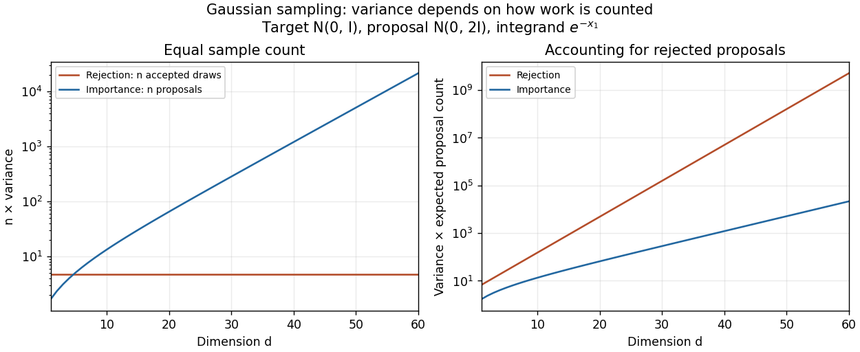
Sample-count and expected-proposal-cost comparisons for the one-coordinate integrand at sigma squared equal to two
. **Details**.

A practical improvement is to exploit the integrand's one-coordinate structure directly: average

e^{- G_{1}}

for standard normal distribution draws

G_{1}

, without generating unused coordinates. The optimal change of proposal distribution in (iii) improves further.

iii

Solution

The integrand is positive, so the minimum-variance importance distribution is its target-weighted probability density function, normalized by

θ = e

q^{⋆} (z) = \frac{e ^{- z_{1}} p ( z )}{e} .

By completing the square,

- z_{1} - \frac{1}{2} z_{1}^{2} - \frac{1}{2} = - \frac{1}{2} (z_{1} + 1)^{2} .

Thus

q^{⋆}

is the multivariate normal distribution

N (- e_{1}, I_{d})

, where

e_{1} = (1, 0, \dots, 0)

is the first standard basis vector. Its importance weight and weighted integrand are

w^{⋆} (z) = e^{z_{1} + 1/2}, w^{⋆} (z) e^{- z_{1}} = e, q min Var (θ_{n}^{IS}) = 0.

A variance cannot be negative, and this proposal makes every summand constant, proving optimality directly. It is admissible under the arbitrary-proposal condition even though its mean vector is not zero. Although optimal proposals usually involve an unknown normalizing integral, here both that integral and the resulting normal distribution are explicit.

2

a

i

Solution

For the exponential distribution with rate

λ

, the cumulative distribution function is

F (x) = 1 - e^{- λ x}

for

x \geq 0

, and zero for

x < 0

. Its quantile function is

F^{- 1} (u) = - \frac{lo g ( 1 - u )}{λ}, 0 < u < 1.

For inverse transform sampling, draw

U

from the uniform distribution on

(0, 1)

and return

- lo g (1 - U) / λ

. Equivalently return

- lo g U / λ

, since

1 - U

has the same uniform distribution. Indeed, for

x \geq 0

P (- lo g U / λ > x) = P (U < e^{- λ x}) = e^{- λ x}

ii

Solution

Integrating the conditional distribution against the exponential distribution probability density function gives, for integer

k \geq 0

P (Y = k) = \int_{0}^{\infty} \frac{e ^{- x} x ^{k}}{k !} λ e^{- λ x} d x = \frac{λ}{k !} \frac{Γ ( k + 1 )}{( 1 + λ ) ^{k + 1}} = \frac{λ}{1 + λ} (\frac{1}{1 + λ})^{k} .

Here the gamma function identity

Γ (k + 1) = k!

evaluates the integral. Hence

Y \sim Geom (\frac{λ}{1 + λ})

{0, 1, 2, \dots}

. Put

r = 1/ (1 + λ)

and

ρ = 1 - r

. The geometric series gives

F (k) = 1 - r^{k + 1}

. Its generalized inverse, the quantile function, is

F^{- 1} (u) = ⌈ \frac{lo g ( 1 - u )}{lo g r} ⌉ - 1, 0 < u < 1.

This is the smallest nonnegative integer

k

for which

1 - r^{k + 1} \geq u

; dividing by

lo g r < 0

reverses the inequality. Draw

U

from the uniform distribution on

(0, 1)

and use this formula. The commonly used expression

⌊ lo g (1 - U) / lo g r ⌋

has the same probability distribution, but differs from the exact generalized inverse when

U

is precisely a jump value of the cumulative distribution function. Such values have probability zero for an ideal continuous uniform draw.

iii

Solution

Write

t = 1 - ρ \in (0, 1)

. The target Poisson distribution and proposal geometric distribution have probability mass functions

p_{k} = e^{- λ} λ^{k} / k!

and

q_{k} = (1 - t) t^{k}

. Their ratio is

R_{k} (t) = \frac{p _{k}}{q _{k}} = \frac{e ^{- λ}}{1 - t} \frac{( λ / t ) ^{k}}{k !} .

The successive ratio

R_{k + 1} / R_{k} = λ / [t (k + 1)]

shows that a maximizing integer is

m = ⌊ λ / t ⌋

, with a tie at

m - 1

when

λ / t

is an integer. Thus the tight envelope is

M (t) = \frac{e ^{- λ}}{1 - t} \frac{( λ / t ) ^{m}}{m !}, m = ⌊ λ / t ⌋ .

For any fixed

t

, draw

Y \sim Geom (1 - t)

using (ii)'s inversion formula with this new parameter, and draw an independent

U

from the uniform distribution on

(0, 1)

. Accept when

U \leq \frac{R _{Y} ( t )}{M ( t )} = \frac{m !}{Y !} (\frac{λ}{t})^{Y - m};

otherwise restart. The acceptance probability is

1/ M (t)

and the expected number of proposals is

M (t)

To minimize that expected count, set

K = ⌈ λ ⌉

. The exact answer is

t_{*} = min {\frac{λ}{K}, \frac{K}{K + 1}}, ρ_{*} = 1 - t_{*} = max {1 - \frac{λ}{K}, \frac{1}{K + 1}} .

Here is a proof that includes the changes of maximizing integer. Each

lo g R_{k} (t)

is a convex function of

t

, since its second derivative is

(1 - t)^{- 2} + k / t^{2} > 0

. Their pointwise maximum

lo g M (t)

is also a convex function. When

m

is fixed its derivative is

\frac{d}{d t} lo g M (t) = \frac{1}{1 - t} - \frac{m}{t} .

(5)

K - 1 < λ \leq K^{2} / (K + 1)

, take

t_{*} = λ / K

, where

m

changes from

K

on the left to

K - 1

on the right. The left derivative is nonpositive because

λ \leq K^{2} / (K + 1)

; the right derivative is nonnegative because

λ \geq K - 1

. This is a minimum. If

K^{2} / (K + 1) < λ \leq K

, take

t_{*} = K / (K + 1)

. There

K < λ / t_{*} \leq K + 1

and the active branch has

m = K

except for the endpoint tie; its derivative vanishes. Convexity again proves the global minimum. The formulas agree at the boundary.

For a fully specified optimal algorithm, compute

K, t_{*}, ρ_{*}

and

m_{*} = ⌊ λ / t_{*} ⌋

once, then use the preceding acceptance test with

t = t_{*}

and

m = m_{*}

. At an integer tie either maximizing integer gives the same test. In code, factorials can be evaluated through the logarithm of the gamma function:

lo g a_{Y} = lo g Γ (m_{*} + 1) - lo g Γ (Y + 1) + (Y - m_{*}) lo g (λ / t_{*}),

(6)

and acceptance is

lo g U \leq min (0, lo g a_{Y})

. This avoids overflowing factorials.

The optimum minimizes expected trials, the usual idealization of time when each proposal and test has constant cost. Actual runtime also depends on the implementation of discrete inversion and factorial evaluation. Simply minimizing an upper bound for

M (t)

would not necessarily give the exact optimum above; see optimal geometric envelope for a Poisson distribution.

b

i

Solution

Because

U \in [0, 1]

, the conditional acceptance probability is

a_{k} = min (1, λ^{k})

, even when the printed threshold exceeds one. Repeating rejected trials gives the clipped acceptance reweighting identity:

P (X = k) = \frac{e ^{- λ} λ ^{k} a _{k} / k !}{\sum _{j \geq 0} e ^{- λ} λ ^{j} a _{j} / j !} .

For

0 < λ < 1

a_{k} = λ^{k}

, including

a_{0} = 1

. The denominator is

e^{- λ} \sum_{k} λ^{2 k} / k! = e^{λ^{2} - λ}

, so

X \sim {Poisson (λ^{2}), Poisson (λ), 0 < λ < 1, λ \geq 1.

For

λ \geq 1

every proposal is accepted, so reweighting by

λ^{k}

would be incorrect. At

λ = 1

both formulas agree. Termination has probability one since the acceptance probability is

e^{λ^{2} - λ} > 0

in the first case and one in the second.

ii

Solution

Define

a_{y} = min {1, λ^{y} /7}

. Given

Y = y

, the direct-return branch has probability

a_{y}

, while the fallback branch distributes its remaining mass uniformly over

0, \dots, y

. The law of total probability therefore gives, for integer

x \geq 0

P (X = x) = e^{- λ} \frac{λ ^{x}}{x !} min {1, \frac{λ ^{x}}{7}} + e^{- λ} y = x \sum \infty \frac{λ ^{y}}{y ! ( y + 1 )} (1 - min {1, \frac{λ ^{y}}{7}}) .

The summation includes

y = x

: a failed direct-return test can still return

x

through the discrete uniform distribution draw. There is no rejection loop and no additional normalization. Summing the displayed probability mass function over

x

gives

\sum_{y} p_{y} [a_{y} + (1 - a_{y}) (y + 1) / (y + 1)] = 1

. At

λ = 1

, for example,

a_{y} = 1/7

at every

y

; it does not become one. This is an instance of the accept-or-fallback mixture identity.

3

a

i

Solution

Let

r = 1 - p

. Since

\frac{d}{d x} lo g (1 - r e^{- β x}) = \frac{β r e ^{- β x}}{1 - r e ^{- β x}},

integration from zero to

x > 0

gives

F (x) = (C / β) [lo g (1 - r e^{- β x}) - lo g p]

. Letting

x \to \infty

and imposing unit total probability gives

C = - \frac{β}{lo g p} > 0, F (x) = ⎩ ⎨ ⎧ 0, 1 - \frac{lo g ( 1 - ( 1 - p ) e ^{- β x} )}{lo g p}, x \leq 0, x > 0.

The probability density function is positive for

x > 0

because

0 < (1 - p) e^{- β x} < 1

. Consequently the cumulative distribution function is increasing, starts at zero and tends to one. This verifies that the derived normalizing constant defines a probability distribution. The family is the exponential-logarithmic distribution with the complementary mixing parameter

r = 1 - p

ii

Solution

Solving

u = F (x)

gives

1 - (1 - p) e^{- β x} = p^{1 - u}

. Hence the quantile function is

F^{- 1} (u) = - \frac{1}{β} lo g (\frac{1 - p ^{1 - u}}{1 - p}), 0 < u < 1.

For such

u

p < p^{1 - u} < 1

, making the logarithm's argument lie in

(0, 1)

and the output positive. Its endpoint limits are

F^{- 1} (0) = 0

and

F^{- 1} (1) = + \infty

. Substitution into (i)'s cumulative distribution function recovers

u

iii

Solution

The following R function performs inverse transform sampling with vectorized numerical computation. It checks finite real scalar parameters, including a nonnegative integer sample count, and gives beta its requested default.

r_sample_f <- function(n, p, beta = 1) {
  scalar <- function(v) {
    is.numeric(v) && !is.complex(v) && length(v) == 1L &&
      is.finite(v)
  }
  if (!scalar(n) || n < 0 || n != floor(n))
    stop("n must be a nonnegative integer")
  if (!scalar(p) || p <= 0 || p >= 1)
    stop("p must lie strictly between 0 and 1")
  if (!scalar(beta) || beta <= 0)
    stop("beta must be positive")
  if (n == 0) return(numeric(0))
  v <- runif(n)
  (log1p(-p) - log(-expm1(v * log(p)))) / beta
}

Here

V = 1 - U

is again a uniform distribution draw, so the expression is the quantile function from (ii). The function expm1(t) evaluates

e^{t} - 1

accurately when

t

is small, avoiding cancellation in

1 - p^{V}

; log1p(-p) evaluates

lo g (1 - p)

. For default bounds, runif excludes both endpoints, so this implementation does not deliberately generate the infinite endpoint of the quantile function. It returns a numeric vector of length n, including an empty vector when n = 0. ^[ref] ^[ref]

b

i

Solution

A numerical power series evaluation needs a stopping rule. For

r = ∣ z ∣ < 1

and integer

a \geq 0

, the absolute remainder after

N

terms satisfies the polylogarithm series remainder bound

Li_{a} (z) - k = 1 \sum N \frac{z ^{k}}{k ^{a}} \leq \frac{r ^{N + 1}}{( N + 1 ) ^{a} ( 1 - r )} .

Indeed

k^{- a} \leq (N + 1)^{- a}

for

k > N

, and the remaining powers sum as a geometric series. This also covers negative

z

. The code sums terms in vectors of at most 4096 entries, checking the bound after each block; there is no loop over individual terms.

polylog <- function(a, z, tol = 1e-10, max_terms = 1000000) {
  scalar <- function(v) {
    is.numeric(v) && !is.complex(v) && length(v) == 1L &&
      is.finite(v)
  }
  if (!scalar(a) || a < 0 || a != floor(a))
    stop("a must be a nonnegative integer")
  if (!scalar(z) || abs(z) >= 1)
    stop("z must be real with abs(z) < 1")
  if (!scalar(tol) || tol <= 0 || tol >= 1)
    stop("tol must lie strictly between 0 and 1")
  if (!scalar(max_terms) || max_terms < 1 ||
      max_terms != floor(max_terms))
    stop("max_terms must be a positive integer")
  if (z == 0) return(0)
  r <- abs(z)
  N <- 0
  ans <- 0
  repeat {
    if (N >= max_terms)
      stop("requested truncation tolerance not reached")
    B <- min(4096, max_terms - N)
    k <- seq.int(N + 1, N + B)
    ans <- ans + sum(z^k * exp(-a * log(k)))
    N <- N + B
    log_bound <- (N + 1) * log(r) - a * log(N + 1) - log1p(-r)
    if (log_bound <= log(tol)) return(ans)
  }
}

This accepts every positive integer order in the question, and also order zero if

0 \in N

is the convention adopted. The bound controls absolute truncation error; floating-point rounding is a separate source of error. Close to

∣ z ∣ = 1

, convergence can be slow. If the resource limit is reached, the function reports failure instead of silently claiming the requested accuracy. Useful exact checks are

Li_{1} (z) = - lo g (1 - z)

and

Li_{0} (z) = z / (1 - z)

ii

Solution

Let

m = E X

and

v = Var (X)

, evaluated from the given polylogarithm formulas. Generate a large sample of independent and identically distributed random variables with r_sample_f, and compute its sample mean

\overline{X}_{n}

and sample variance

S_{n}^{2}

using mean and var. The central limit theorem gives the first standardized check:

Z_{m} = \frac{n ( X _{n} - m )}{v} \Rightarrow N (0, 1) .

For the second check, the correct asymptotic variance of the sample variance involves the fourth central moment

μ_{4} = E [(X - m)^{4}]

Z_{v} = \frac{n ( S _{n}^{2} - v )}{μ _{4} - v ^{2}} \Rightarrow N (0, 1) .

The denominator is not

2 v^{2}

unless the probability distribution has the requisite fourth central moment, as does the normal distribution. Here the probability density function decays exponentially, so all required moments are finite.

To compute

μ_{4}

, expand the denominator of the probability density function as a geometric series and integrate each nonnegative term. The gamma function integral gives the raw moments

m_{j} := E [X^{j}] = - \frac{j ! Li _{j + 1} ( 1 - p )}{β ^{j} l o g p}, j \geq 1.

Thus

v = m_{2} - m_{1}^{2}

and

μ_{4} = m_{4} - 4 m_{1} m_{3} + 6 m_{1}^{2} m_{2} - 3 m_{1}^{4}

. The following R code implements both checks for chosen interior parameters and large n:

p <- 0.4
beta <- 1.3
n <- 100000
raw_m <- vapply(1:4, function(j) {
  -factorial(j) * polylog(j + 1, 1 - p) / (beta^j * log(p))
}, numeric(1))
m <- raw_m[1]
v <- raw_m[2] - m^2
mu4 <- raw_m[4] - 4 * m * raw_m[3] +
  6 * m^2 * raw_m[2] - 3 * m^4
x <- r_sample_f(n, p, beta)
c(mean_check = sqrt(n) * (mean(x) - m) / sqrt(v),
  variance_check = sqrt(n) * (var(x) - v) / sqrt(mu4 - v^2))

For each check separately, an absolute value below

1.96

is consistent with its approximate

95%

confidence interval. Repeat with many independent samples: the two standardized statistics should each resemble a standard normal distribution, with about

5%

outside that range. Also vary

p

β

and n; a systematic discrepancy that grows with

n

suggests a bias. The two checks from the same sample are generally dependent, so passing both is not itself a joint

95%

statement, nor can a finite test prove that a generator is correct.

The second central limit theorem follows from the central limit theorem for the sample variance:

n (S_{n}^{2} - v)

differs by a quantity tending to zero in probability from

n^{- 1/2} \sum_{i} [(X_{i} - m)^{2} - v]

ℓ (p, β; x) = n {lo g β - lo g (- lo g p) + lo g (1 - p)} - β i = 1 \sum n x_{i} - i = 1 \sum n lo g (1 - (1 - p) e^{- β x_{i}}) .