Past exam of the simulation and statistical programming course of the University of Oxford / 2021 (A12, A13766W1)

a

Solution

Write

s = σ^{2} \geq 1

. The two multivariate normal distribution probability density functions have ratio

w (x) = \frac{p ( x )}{q ( x )} = s^{d /2} exp [- \frac{1}{2} (1 - s^{- 1}) ∥ x ∥^{2}] .

Here

∥ x ∥

is the Euclidean norm. Consequently the smallest rejection sampling envelope constant, and its acceptance probability, are

M_{*} = x sup w (x) = s^{d /2} = σ^{d}, P (accept) = s^{- d /2} .

The supremum is attained at

x = 0

; hence no smaller constant can dominate the ratio. Draw

Y \sim N (0, s I_{d})

and an independent

U

from the uniform distribution on

(0, 1)

. Accept

Y

when

U \leq exp [- \frac{1}{2} (1 - s^{- 1}) ∥ Y ∥^{2}];

otherwise repeat with fresh independent random variables. One can generate

Y = s G

using a random vector

G

with independent standard normal distribution coordinates.

For any measurable set

B

, the joint acceptance probability is

\int_{B} q (y) p (y) / (M_{*} q (y)) d y = M_{*}^{- 1} \int_{B} p (y) d y

. Dividing by

1/ M_{*}

proves that the returned random vector has probability density function

p

. The number of proposals has a geometric distribution on the positive integers, with expected value

M_{*}

. When

s = 1

, every proposal is accepted.

b

Solution

The moment-generating function of a standard normal distribution gives

E [e^{t X_{j}}] = e^{t^{2} /2}

. Using independence of the coordinates,

θ = E_{p} [ϕ (X)] = \prod_{j = 1}^{d} E [e^{- X_{j}}] = e^{d /2}, E_{p} [ϕ (X)^{2}] = \prod_{j = 1}^{d} E [e^{- 2 X_{j}}] = e^{2 d} .

The accepted draws are independent and identically distributed random variables, so their sample mean is an unbiased estimator and has variance

Var (θ_{n}^{RS}) = \frac{e ^{2 d} - e ^{d}}{n} .

This counts

n

accepted draws, requiring

n σ^{d}

proposals in expectation.

c

Solution

An importance weight has expected value

E_{q} [w (Z)] = \int p (z) d z = 1

. From the ratio in (a),

E_{q} [w (Z)^{2}] = s^{d} \prod_{j = 1}^{d} E_{Z_{j} \sim N (0, s)} [e^{- (1 - s^{- 1}) Z_{j}^{2}}] .

The supplied normal distribution transform applies with quadratic coefficient

- (1 - s^{- 1})

, giving each factor

(2 s - 1)^{- 1/2}

. Thus

Var_{q} (w (Z)) = (\frac{s}{2 s - 1})^{d} - 1.

For

s > 1

, the base

A := s / 2 s - 1

exceeds one because

s^{2} - (2 s - 1) = (s - 1)^{2} > 0

: importance weight variance increases exponentially with dimension. For

s = 1

, the importance weight is identically one and its variance is zero. This calculation concerns the importance weight, rather than the weighted integrand.

d

i

Solution

For the new integrand,

θ = E_{p} [e^{- X_{1}}] = e^{1/2}

and

Var_{p} (e^{- X_{1}}) = e^{2} - e

, independently of dimension. Chebyshev's inequality therefore yields

P (∣ θ_{n}^{RS} - θ ∣ \geq ε) \leq \frac{e ^{2} - e}{n ε ^{2}} .

A sufficient positive integer sample count is

n = ⌈ \frac{e ^{2} - e}{δ ε ^{2}} ⌉ .

The ceiling function ensures that the bound is at most

δ

, so the strict-error event in the question has probability at least

1 - δ

. The required number of accepted draws is independent of

d

; their expected proposal count is

n σ^{d}

ii

Solution

At equal sample count, rejection sampling eventually has smaller variance for fixed $σ^{2} > 1$ ; at equal expected proposal cost, importance sampling eventually wins. The distinction matters because a sample of the rejection sampling estimator means an accepted draw.

For the importance sampling estimator, all coordinates contribute to the importance weight although only one enters the integrand. The same normal distribution transform as in (c), now with linear coefficient

- 2

for coordinate one, gives

E_{q} [(w (Z) e^{- Z_{1}})^{2}] = A^{d} exp (\frac{2 s}{2 s - 1}), A = \frac{s}{2 s - 1} .

Both estimators are unbiased estimators of

e

, and

Var (θ_{n}^{IS}) = \frac{A ^{d} e ^{2 s / (2 s - 1)} - e}{n}, Var (θ_{n}^{RS}) = \frac{e ^{2} - e}{n} .

For fixed

s > 1

, the first variance grows exponentially while the second stays constant. This is the benefit of returning exact target draws in rejection sampling. However, obtaining those draws costs

s^{d /2}

proposals each on average.

To compare computational work, multiply each variance by its expected proposal count. For importance sampling that count is

n

; for rejection sampling it is

n s^{d /2}

. The ratio of the resulting cost-normalized variances is

\frac{A ^{d} e ^{2 s / (2 s - 1)} - e}{s ^{d /2} ( e ^{2} - e )} ⟶ 0 (d \to \infty),

because

A / s = s / (2 s - 1) < 1

. Thus importance sampling eventually gives better precision for the same expected number of proposals, assuming comparable work per proposal. This is an asymptotic cost comparison, not a guarantee that a fixed small computing budget produces any accepted draws. Both methods still deteriorate exponentially in this comparison. For

s = 1

they coincide and every proposal is accepted.

Figure 1.
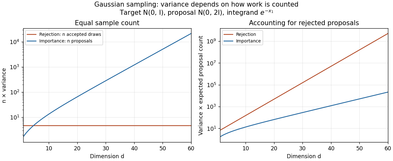
Sample-count and expected-proposal-cost comparisons for the one-coordinate integrand at sigma squared equal to two
. **Details**.

A practical improvement is to exploit the integrand's one-coordinate structure directly: average

e^{- G_{1}}

for standard normal distribution draws

G_{1}

, without generating unused coordinates. The optimal change of proposal distribution in (iii) improves further.

iii

Solution

The integrand is positive, so the minimum-variance importance distribution is its target-weighted probability density function, normalized by

θ = e

q^{⋆} (z) = \frac{e ^{- z_{1}} p ( z )}{e} .

By completing the square,

- z_{1} - \frac{1}{2} z_{1}^{2} - \frac{1}{2} = - \frac{1}{2} (z_{1} + 1)^{2} .

Thus

q^{⋆}

is the multivariate normal distribution

N (- e_{1}, I_{d})

, where

e_{1} = (1, 0, \dots, 0)

is the first standard basis vector. Its importance weight and weighted integrand are

w^{⋆} (z) = e^{z_{1} + 1/2}, w^{⋆} (z) e^{- z_{1}} = e, q min Var (θ_{n}^{IS}) = 0.

A variance cannot be negative, and this proposal makes every summand constant, proving optimality directly. It is admissible under the arbitrary-proposal condition even though its mean vector is not zero. Although optimal proposals usually involve an unknown normalizing integral, here both that integral and the resulting normal distribution are explicit.

2

a

i

Solution

For the exponential distribution with rate

λ

, the cumulative distribution function is

F (x) = 1 - e^{- λ x}

for

x \geq 0

, and zero for

x < 0

. Its quantile function is

F^{- 1} (u) = - \frac{lo g ( 1 - u )}{λ}, 0 < u < 1.

For inverse transform sampling, draw

U

from the uniform distribution on

(0, 1)

and return

- lo g (1 - U) / λ

. Equivalently return

- lo g U / λ

, since

1 - U

has the same uniform distribution. Indeed, for

x \geq 0

P (- lo g U / λ > x) = P (U < e^{- λ x}) = e^{- λ x}

ii

Solution

Integrating the conditional distribution against the exponential distribution probability density function gives, for integer

k \geq 0

P (Y = k) = \int_{0}^{\infty} \frac{e ^{- x} x ^{k}}{k !} λ e^{- λ x} d x = \frac{λ}{k !} \frac{Γ ( k + 1 )}{( 1 + λ ) ^{k + 1}} = \frac{λ}{1 + λ} (\frac{1}{1 + λ})^{k} .

Here the gamma function identity

Γ (k + 1) = k!

evaluates the integral. Hence

Y \sim Geom (\frac{λ}{1 + λ})

{0, 1, 2, \dots}

. Put

r = 1/ (1 + λ)

and

ρ = 1 - r

. The geometric series gives

F (k) = 1 - r^{k + 1}

. Its generalized inverse, the quantile function, is

F^{- 1} (u) = ⌈ \frac{lo g ( 1 - u )}{lo g r} ⌉ - 1, 0 < u < 1.

This is the smallest nonnegative integer

k

for which

1 - r^{k + 1} \geq u

; dividing by

lo g r < 0

reverses the inequality. Draw

U

from the uniform distribution on

(0, 1)

and use this formula. The commonly used expression

⌊ lo g (1 - U) / lo g r ⌋

has the same probability distribution, but differs from the exact generalized inverse when

U

is precisely a jump value of the cumulative distribution function. Such values have probability zero for an ideal continuous uniform draw.

iii

Solution

Write

t = 1 - ρ \in (0, 1)

. The target Poisson distribution and proposal geometric distribution have probability mass functions

p_{k} = e^{- λ} λ^{k} / k!

and

q_{k} = (1 - t) t^{k}

. Their ratio is

R_{k} (t) = \frac{p _{k}}{q _{k}} = \frac{e ^{- λ}}{1 - t} \frac{( λ / t ) ^{k}}{k !} .

The successive ratio

R_{k + 1} / R_{k} = λ / [t (k + 1)]

shows that a maximizing integer is

m = ⌊ λ / t ⌋

, with a tie at

m - 1

when

λ / t

is an integer. Thus the tight envelope is

M (t) = \frac{e ^{- λ}}{1 - t} \frac{( λ / t ) ^{m}}{m !}, m = ⌊ λ / t ⌋ .

For any fixed

t

, draw

Y \sim Geom (1 - t)

using (ii)'s inversion formula with this new parameter, and draw an independent

U

from the uniform distribution on

(0, 1)

. Accept when

U \leq \frac{R _{Y} ( t )}{M ( t )} = \frac{m !}{Y !} (\frac{λ}{t})^{Y - m};

otherwise restart. The acceptance probability is

1/ M (t)

and the expected number of proposals is

M (t)

To minimize that expected count, set

K = ⌈ λ ⌉

. The exact answer is

t_{*} = min {\frac{λ}{K}, \frac{K}{K + 1}}, ρ_{*} = 1 - t_{*} = max {1 - \frac{λ}{K}, \frac{1}{K + 1}} .

(4)

Here is a proof that includes the changes of maximizing integer. Each

lo g R_{k} (t)

is a convex function of

t

, since its second derivative is

(1 - t)^{- 2} + k / t^{2} > 0

. Their pointwise maximum

lo g M (t)

is also a convex function. When

m

is fixed its derivative is

\frac{d}{d t} lo g M (t) = \frac{1}{1 - t} - \frac{m}{t} .

(5)

K - 1 < λ \leq K^{2} / (K + 1)

, take

t_{*} = λ / K

, where

m

changes from

K

on the left to

K - 1

on the right. The left derivative is nonpositive because

λ \leq K^{2} / (K + 1)

; the right derivative is nonnegative because

λ \geq K - 1

. This is a minimum. If

K^{2} / (K + 1) < λ \leq K

, take

t_{*} = K / (K + 1)

. There

K < λ / t_{*} \leq K + 1

and the active branch has

m = K

except for the endpoint tie; its derivative vanishes. Convexity again proves the global minimum. The formulas agree at the boundary.

For a fully specified optimal algorithm, compute

K, t_{*}, ρ_{*}

and

m_{*} = ⌊ λ / t_{*} ⌋

once, then use the preceding acceptance test with

t = t_{*}

and

m = m_{*}

. At an integer tie either maximizing integer gives the same test. In code, factorials can be evaluated through the logarithm of the gamma function:

lo g a_{Y} = lo g Γ (m_{*} + 1) - lo g Γ (Y + 1) + (Y - m_{*}) lo g (λ / t_{*}),

(6)

and acceptance is

lo g U \leq min (0, lo g a_{Y})

. This avoids overflowing factorials.

The optimum minimizes expected trials, the usual idealization of time when each proposal and test has constant cost. Actual runtime also depends on the implementation of discrete inversion and factorial evaluation. Simply minimizing an upper bound for

M (t)

would not necessarily give the exact optimum above; see optimal geometric envelope for a Poisson distribution.

b

i

Solution

Because

U \in [0, 1]

, the conditional acceptance probability is

a_{k} = min (1, λ^{k})

, even when the printed threshold exceeds one. Repeating rejected trials gives the clipped acceptance reweighting identity:

P (X = k) = \frac{e ^{- λ} λ ^{k} a _{k} / k !}{\sum _{j \geq 0} e ^{- λ} λ ^{j} a _{j} / j !} .

For

0 < λ < 1

a_{k} = λ^{k}

, including

a_{0} = 1

. The denominator is

e^{- λ} \sum_{k} λ^{2 k} / k! = e^{λ^{2} - λ}

, so

X \sim {Poisson (λ^{2}), Poisson (λ), 0 < λ < 1, λ \geq 1.

For

λ \geq 1

every proposal is accepted, so reweighting by

λ^{k}

would be incorrect. At

λ = 1

both formulas agree. Termination has probability one since the acceptance probability is

e^{λ^{2} - λ} > 0

in the first case and one in the second.

ii

Solution

Define

a_{y} = min {1, λ^{y} /7}

. Given

Y = y

, the direct-return branch has probability

a_{y}

, while the fallback branch distributes its remaining mass uniformly over

0, \dots, y

. The law of total probability therefore gives, for integer

x \geq 0

P (X = x) = e^{- λ} \frac{λ ^{x}}{x !} min {1, \frac{λ ^{x}}{7}} + e^{- λ} y = x \sum \infty \frac{λ ^{y}}{y ! ( y + 1 )} (1 - min {1, \frac{λ ^{y}}{7}}) .

The summation includes

y = x

: a failed direct-return test can still return

x

through the discrete uniform distribution draw. There is no rejection loop and no additional normalization. Summing the displayed probability mass function over

x

gives

\sum_{y} p_{y} [a_{y} + (1 - a_{y}) (y + 1) / (y + 1)] = 1

. At

λ = 1

, for example,

a_{y} = 1/7

at every

y

; it does not become one. This is an instance of the accept-or-fallback mixture identity.

3

a

i

Solution

Let

r = 1 - p

. Since

\frac{d}{d x} lo g (1 - r e^{- β x}) = \frac{β r e ^{- β x}}{1 - r e ^{- β x}},

integration from zero to

x > 0

gives

F (x) = (C / β) [lo g (1 - r e^{- β x}) - lo g p]

. Letting

x \to \infty

and imposing unit total probability gives

C = - \frac{β}{lo g p} > 0, F (x) = ⎩ ⎨ ⎧ 0, 1 - \frac{lo g ( 1 - ( 1 - p ) e ^{- β x} )}{lo g p}, x \leq 0, x > 0.

The probability density function is positive for

x > 0

because

0 < (1 - p) e^{- β x} < 1

. Consequently the cumulative distribution function is increasing, starts at zero and tends to one. This verifies that the derived normalizing constant defines a probability distribution. The family is the exponential-logarithmic distribution with the complementary mixing parameter

r = 1 - p

ii

Solution

Solving

u = F (x)

gives

1 - (1 - p) e^{- β x} = p^{1 - u}

. Hence the quantile function is

F^{- 1} (u) = - \frac{1}{β} lo g (\frac{1 - p ^{1 - u}}{1 - p}), 0 < u < 1.

For such

u

p < p^{1 - u} < 1

, making the logarithm's argument lie in

(0, 1)

and the output positive. Its endpoint limits are

F^{- 1} (0) = 0

and

F^{- 1} (1) = + \infty

. Substitution into (i)'s cumulative distribution function recovers

u

iii

Solution

The following R function performs inverse transform sampling with vectorized numerical computation. It checks finite real scalar parameters, including a nonnegative integer sample count, and gives beta its requested default.

r_sample_f <- function(n, p, beta = 1) {
  scalar <- function(v) {
    is.numeric(v) && !is.complex(v) && length(v) == 1L &&
      is.finite(v)
  }
  if (!scalar(n) || n < 0 || n != floor(n))
    stop("n must be a nonnegative integer")
  if (!scalar(p) || p <= 0 || p >= 1)
    stop("p must lie strictly between 0 and 1")
  if (!scalar(beta) || beta <= 0)
    stop("beta must be positive")
  if (n == 0) return(numeric(0))
  v <- runif(n)
  (log1p(-p) - log(-expm1(v * log(p)))) / beta
}

Here

V = 1 - U

is again a uniform distribution draw, so the expression is the quantile function from (ii). The function expm1(t) evaluates

e^{t} - 1

accurately when

t

is small, avoiding cancellation in

1 - p^{V}

; log1p(-p) evaluates

lo g (1 - p)

. For default bounds, runif excludes both endpoints, so this implementation does not deliberately generate the infinite endpoint of the quantile function. It returns a numeric vector of length n, including an empty vector when n = 0. ^[ref] ^[ref]

b

i

Solution

A numerical power series evaluation needs a stopping rule. For

r = ∣ z ∣ < 1

and integer

a \geq 0

, the absolute remainder after

N

terms satisfies the polylogarithm series remainder bound

Li_{a} (z) - k = 1 \sum N \frac{z ^{k}}{k ^{a}} \leq \frac{r ^{N + 1}}{( N + 1 ) ^{a} ( 1 - r )} .

Indeed

k^{- a} \leq (N + 1)^{- a}

for

k > N

, and the remaining powers sum as a geometric series. This also covers negative

z

. The code sums terms in vectors of at most 4096 entries, checking the bound after each block; there is no loop over individual terms.

polylog <- function(a, z, tol = 1e-10, max_terms = 1000000) {
  scalar <- function(v) {
    is.numeric(v) && !is.complex(v) && length(v) == 1L &&
      is.finite(v)
  }
  if (!scalar(a) || a < 0 || a != floor(a))
    stop("a must be a nonnegative integer")
  if (!scalar(z) || abs(z) >= 1)
    stop("z must be real with abs(z) < 1")
  if (!scalar(tol) || tol <= 0 || tol >= 1)
    stop("tol must lie strictly between 0 and 1")
  if (!scalar(max_terms) || max_terms < 1 ||
      max_terms != floor(max_terms))
    stop("max_terms must be a positive integer")
  if (z == 0) return(0)
  r <- abs(z)
  N <- 0
  ans <- 0
  repeat {
    if (N >= max_terms)
      stop("requested truncation tolerance not reached")
    B <- min(4096, max_terms - N)
    k <- seq.int(N + 1, N + B)
    ans <- ans + sum(z^k * exp(-a * log(k)))
    N <- N + B
    log_bound <- (N + 1) * log(r) - a * log(N + 1) - log1p(-r)
    if (log_bound <= log(tol)) return(ans)
  }
}

This accepts every positive integer order in the question, and also order zero if

0 \in N

is the convention adopted. The bound controls absolute truncation error; floating-point rounding is a separate source of error. Close to

∣ z ∣ = 1

, convergence can be slow. If the resource limit is reached, the function reports failure instead of silently claiming the requested accuracy. Useful exact checks are

Li_{1} (z) = - lo g (1 - z)

and

Li_{0} (z) = z / (1 - z)

ii

Solution

Let

m = E X

and

v = Var (X)

, evaluated from the given polylogarithm formulas. Generate a large sample of independent and identically distributed random variables with r_sample_f, and compute its sample mean

\overline{X}_{n}

and sample variance

S_{n}^{2}

using mean and var. The central limit theorem gives the first standardized check:

Z_{m} = \frac{n ( X _{n} - m )}{v} \Rightarrow N (0, 1) .

For the second check, the correct asymptotic variance of the sample variance involves the fourth central moment

μ_{4} = E [(X - m)^{4}]

Z_{v} = \frac{n ( S _{n}^{2} - v )}{μ _{4} - v ^{2}} \Rightarrow N (0, 1) .

The denominator is not

2 v^{2}

unless the probability distribution has the requisite fourth central moment, as does the normal distribution. Here the probability density function decays exponentially, so all required moments are finite.

To compute

μ_{4}

, expand the denominator of the probability density function as a geometric series and integrate each nonnegative term. The gamma function integral gives the raw moments

m_{j} := E [X^{j}] = - \frac{j ! Li _{j + 1} ( 1 - p )}{β ^{j} l o g p}, j \geq 1.

Thus

v = m_{2} - m_{1}^{2}

and

μ_{4} = m_{4} - 4 m_{1} m_{3} + 6 m_{1}^{2} m_{2} - 3 m_{1}^{4}

. The following R code implements both checks for chosen interior parameters and large n:

p <- 0.4
beta <- 1.3
n <- 100000
raw_m <- vapply(1:4, function(j) {
  -factorial(j) * polylog(j + 1, 1 - p) / (beta^j * log(p))
}, numeric(1))
m <- raw_m[1]
v <- raw_m[2] - m^2
mu4 <- raw_m[4] - 4 * m * raw_m[3] +
  6 * m^2 * raw_m[2] - 3 * m^4
x <- r_sample_f(n, p, beta)
c(mean_check = sqrt(n) * (mean(x) - m) / sqrt(v),
  variance_check = sqrt(n) * (var(x) - v) / sqrt(mu4 - v^2))

For each check separately, an absolute value below

1.96

is consistent with its approximate

95%

confidence interval. Repeat with many independent samples: the two standardized statistics should each resemble a standard normal distribution, with about

5%

outside that range. Also vary

p

β

and n; a systematic discrepancy that grows with

n

suggests a bias. The two checks from the same sample are generally dependent, so passing both is not itself a joint

95%

statement, nor can a finite test prove that a generator is correct.

The second central limit theorem follows from the central limit theorem for the sample variance:

n (S_{n}^{2} - v)

differs by a quantity tending to zero in probability from

n^{- 1/2} \sum_{i} [(X_{i} - m)^{2} - v]

c

i

Solution

Taking the logarithm of the normalized probability density function, then summing over the independent observations, gives the log-likelihood

ℓ (p, β; x) = n {lo g β - lo g (- lo g p) + lo g (1 - p)} - β i = 1 \sum n x_{i} - i = 1 \sum n lo g (1 - (1 - p) e^{- β x_{i}}) .

Both

p

and

β

are parameters being inferred, so their contributions to the normalizing constant must be retained. The following R implementation validates the arguments and returns one number:

ll_f <- function(p, beta, x) {
  scalar <- function(v) {
    is.numeric(v) && !is.complex(v) && length(v) == 1L &&
      is.finite(v)
  }
  if (!scalar(p) || p <= 0 || p >= 1)
    stop("p must lie strictly between 0 and 1")
  if (!scalar(beta) || beta <= 0)
    stop("beta must be positive")
  if (!is.numeric(x) || is.complex(x) || !is.null(dim(x)) ||
      any(!is.finite(x)) || any(x <= 0))
    stop("x must be a vector of finite positive numbers")
  if (length(x) == 0L) return(0)
  t <- log1p(-p) - beta * x
  length(x) * (log(beta) - log(-log(p))) +
    sum(t - log(-expm1(t)))
}

Here

t_{i} = lo g (1 - p) - β x_{i} < 0

and -expm1(t) computes

1 - e^{t}

accurately near zero. The empty-data likelihood function is one, so its log-likelihood is zero. Invalid parameter values produce errors in this evaluator; the next algorithm rejects candidates outside the parameter support before calling it.

ii

Solution

Assume

a, b, μ > 0

and a current state with

0 < p < 1

β > 0

. The unnormalized posterior density is

π (p, β ∣ x) \propto exp {ℓ (p, β; x)} p^{a - 1} (1 - p)^{b - 1} μ^{- 1} e^{- β / μ} .

Thus the log-posterior, up to an additive constant, is the log-likelihood plus the beta distribution and exponential distribution log prior densities. The exponential distribution rate is

1/ μ

, since

μ

is its mean. ^[ref] ^[ref]

Choose a symmetric joint random-walk Metropolis algorithm proposal:

p^{'} = p + 0.1 G_{1}

and

β^{'} = β + (μ /2) G_{2}

, for independent standard normal distribution draws. Its scale depends only on fixed hyperparameters, so forward and reverse proposal probability density functions agree. Reject immediately outside

(0, 1) \times (0, \infty)

; otherwise accept with Metropolis–Hastings acceptance probability

α = min {1, exp [lo g π (p^{'}, β^{'} ∣ x) - lo g π (p, β ∣ x)]} .

The following function makes exactly one proposal, with rejection retaining both old parameters:

MHstep <- function(x, p, beta, a, b, mu) {
  p_new <- rnorm(1, mean = p, sd = 0.1)
  beta_new <- rnorm(1, mean = beta, sd = mu / 2)
  if (p_new <= 0 || p_new >= 1 || beta_new <= 0)
    return(list(p = p, theta = beta))
  logpost <- function(pp, bb) {
    ll_f(pp, bb, x) + dbeta(pp, a, b, log = TRUE) +
      dexp(bb, rate = 1 / mu, log = TRUE)
  }
  logA <- logpost(p_new, beta_new) - logpost(p, beta)
  if (log(runif(1)) <= min(0, logA)) {
    p <- p_new
    beta <- beta_new
  }
  list(p = p, theta = beta)
}

The returned field theta contains the updated value of beta. The original PDF really asks for p and theta, although no parameter

θ

is defined in this question. This choice preserves its literal interface while making the intended second parameter explicit. A caller therefore advances with state <- MHstep(x, p, beta, a, b, mu), p <- state$p, and beta <- state$theta.

The proposal is an unrestricted symmetric normal distribution followed by rejection outside the support. Repeatedly drawing until a valid proposal appears would instead truncate and renormalize the proposal, requiring a proposal-density correction. The code uses immediate rejection and needs no such correction. The displayed scales are valid fixed choices; practical efficiency can be improved using a separate tuning phase.

iii

Solution